
Weather
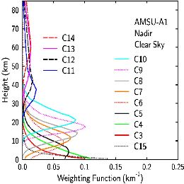
Ralf Bennartz from the University of Wisconsin gives an introduction on the principles of atmospheric soundings with AIRS and AMSU sensors.
High resolution infrared sounders, such as AIRS and IASI, and microwave sounders, such as AMSU, are a key element of the global satellite observing system and provide a wealth of data important for various operational applications including data assimilation and nowcasting applications. This presentation will revisit the physical basis of infrared and microwave sounding and provide an overview on the state-of-the-art of microwave and infrared soundings.
Nuno Moreira from IPMA guides you through the web sites mentioned in the presentations during the Polar Satellites Week.
In this session you will be taken on a website tour, visiting pages where polar satellite products referred during the whole EUMETRAIN Polar Satellite Week can be visualized. “Web-Visits” will naturally include EUMETSAT or NOAA pages and it will be an opportunity to make a wrap-up on the contents previously discussed...
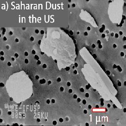
Piet Stammes from KNMI talks about aerosol retrieval with GOME-2 instrument onboard MetOp satellites since 2006. Intercomparison with other instrument data and examples round up the presentation.
Aerosols are small liquid or solid particles in the atmosphere, like soil dust, sulphate and nitrate droplets, organic compounds, volcanic ash, etc.. Aerosols affect weather and climate by reflection and absorption of sunlight, by affecting cloud formation and precipitation, and by reducing visibility. Satellite detection of aerosols is often difficult because of the relatively weak reflectance of aerosols as compared to clouds and the background reflection of the underlying surface. Using UV-Visible spectrometers like OMI and GOME-2, UV absorbing aerosols like biomass burning smoke, volcanic ash and desert dust can be detected, even in cloudy cases and over land surfaces. In this presentation the current and future aerosol products from GOME-2 available from the O3MSAF will be introduced.
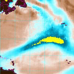
NOAA satellite analyst Sheldon Kusselson shows the variety of water vapour products available from polar platforms. A practical example concludes his presentation.
Since 1992 operational NOAA satellite analysts and forecasters have used polar orbiting microwave products to complement and supplement geostationary satellite, observational and computer model data to further improve precipitation forecasts. My session will provide an overview of current SSMIS and NOAA/MetOp MHS and AMSU polar orbiting microwave products, like Total Precipitable Water (TPW) and Rain Rate (RR) and how they can be used to help enhance precipitation forecasts with an emphasis on the eastern North Atlantic Ocean into the European continent. From these different individual satellite sensors microwave TPW and RR products have come a new class of satellite product called “the blended or merged product” that will also be discussed, displayed and compared with EUMETSAT geostationary satellite imagery. A case study showing these blended/merged TPW and RR products for the February 2010 Madeira storm will also be shown.
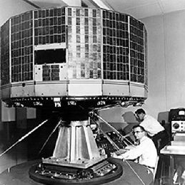
Steve Ackerman gives an introduction on cloud detection methods used to segregate cloud free from cloud contaminated satellite pixel.
Early in the history of polar orbiting satellite, imaging instruments were included to detect and classify clouds. Steve Ackerman will begin with a brief historical look at these first observations. This presentation will discuss the types of algorithms developed and applied to visible and infrared observations from the NOAA series, the two NASA EOS and the EUMETSAT MetOp platforms. Steve Ackerman will discuss areas of strength and weakness in cloud detection from these platforms and will end by exploring some climate and regional applications of the cloud analyzes from some of these cloud images.
Stefania De Angelis shows in her presentation the different categories of Hydro-SAF precipitation products derived from polar orbiting satellite data.
Monitoring and measurement of precipitation from satellite is an important capability for many types of users, such as the Meteorological Services, Hydro-geological Services and the structures of civil protection. The consortium H-SAF, within EUMETSAT, has among its objectives to provide continuous operational products for instantaneous measurement of rainfall using data from microwave instruments, on-board polar satellites, in synergy with the infrared data of the geostationary satellite MSG. In addition to the production operation, the HSAF provides validation service on each product and carries out independent validation of the benefits of the novel H-SAF satellite-derived data on hydrological practical applications.
Adam Dybbroe presents Nowcasting SAF products developed for polar satellites. He gives an overview on existing and future products retrieved from MetOp and NPP satellite data.
The EUMETSAT SAF to support Nowcasting (NWCSAF) develops two software packages, one for Geostationary imagery and one for polar satellite imagery. Both packages retrieve Cloud and other parameters relevant for Nowcasting and short range forecasting. The Polar Platform System (PPS) software package retrieves information on clouds and precipitation. The parameters/products derived are, Cloud Mask, Cloud Type, Cloud Top Temperature and Height, Precipitating Clouds, and a number of cloud microphysical parameters (e.g. liquid water path and cloud phase). The first version of PPS was released in 2004, and it was originally developed to run on local direct readout data from NOAA and Metop (AVHRR and AMSU/MHS). But recently it has been extended to run also on NPP/VIIRS data. And PPS is now also capable of running on many different data formats and services. It is currently being introduced on the EARS Network to run on NOAA19 and Metop-A. In this presentation Adam Dybbroe will give an overview of how PPS works, but the main focus will be on the parameters and products that can be derived with PPS, and how they can be used in Nowcasting applications.
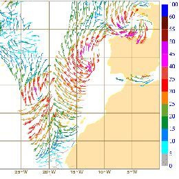
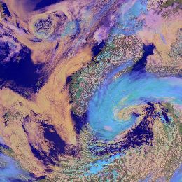
Storm Xynthia developed over the North Atlantic in late February 2010. The ASCAT sensor of EUMETSAT MetOp-A satellite tracked its evolution and provided insight into the life cycle of the storm.
In this presentation Nuno Moreira talks about Xynthia, a storm that affected North Atlantic and Europe in the end of February 2010. He focuses on the cyclogenesis process, which fits the classification of a "bomb", and on the remote observations of the storm. This observation does not only cover MSG imagery, but also ASCAT wind data and derived mean sea level pressure estimates. The advantages and disadvantages of using ASCAT wind in nowcasting for this kind of storms is also discussed.
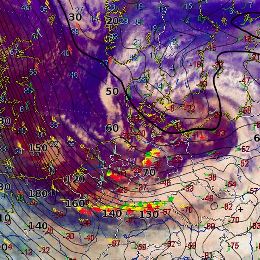
The presenter gives an overview into the mechanisms of convective lines connected to winter storms such as Emma.
Convective lines in connection with intense cyclogenesis hit Middle and Western Europe almost every winter season. These lines move very quickly and are often connected with thunderstorms, heavy gusts and graupel or even hail. In this presentation the related conceptual model and the preconvective environment will be explained. Based upon different satellite products and additional data two examples will be discussed.
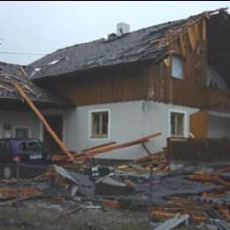
Presentation of Winter-Storm Emma which severely affected Central Europe with heavy downbursts and thunderstorms.
On 1 March 2008, the powerful late winter cyclone Emma caused widespread damage and claimed 14 lives in Central Europe. Embedded in the synoptic-scale storm field, deep convection along the cold front played a significant role in further enhancing the wind gusts. This presentation aims to unfurl an outstanding case of a rapid cyclogenesis, to match the events at the earth's surface with the storm structures seen in satellite and radar data, and finally to track down possible mechanisms which may have contributed to paving the way for one of the strongest downbursts ever documented worldwide.
The presenter analyses the mesoscale synoptic situation of medicanes from the past decades. He focuses on similarities in NWP fields.
The Mediterranean area can be affected by particular cyclones characterized by an unusual life cycle. This life cycle can be divided into two distinct parts: in the initial part the subject has a warm core and an asymmetric structure, which are typical aspects of a tropical storm. In the second part, it evolves rather like a cyclone of middle latitudes, usually explained by the classical theories; its origin is either on the sea as on the desert. These entities generally include extreme events, such as intense convection, strong winds and coastal storm surges; consequently, they assume a significant importance in the diagnostic and forecasting. This lecture will explain the energy contributions and the thermodynamic processes involved in the entire evolution, also describing the various significant aspects making use of adapted diagnostic procedures.
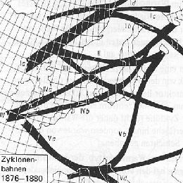
Kristian Horvath from the Croatian Met-Service focuses in his presentation on the different types of cyclogenesis in the Mediterranean Bassin.
The classification of cyclones and their tracks in the Mediterranean will be presented, with a special attention on the lee cyclones and their tracks when moving farther from the initiation area. Furthermore, the atmospheric ingredients at play during lee cyclone formation and development will be reviewed, such as the crucial role of the upper-level dynamical factors, but also the near-surface lee-side thermal or potential vorticity (PV) anomalies and surface fluxes, including their interactions with the orography and mutual non-linear synergies. In addition, the use of “PV thinking” will be demonstrated for easier conceptual understanding of the formation mechanisms. The results of numerical studies show that the intensity and track of lee cyclones are very sensitive to the details of the upper-level trough, such as its exact position relative to the mountain, the intensity and existence of sub-synoptic vorticity cores, which may result in reducing the predictability of lee cyclones in the Mediterranean area.