Chapter III: The days before heavy rain are significant for flood formation
Table of Contents
- Chapter III: The days before heavy rain are significant for flood formation
- Introduction
- Weather in the days before the flood
- The significance of extreme soil moisture at the end of May 2013
- The influence of snow cover
Introduction
Each German state has a responsibility to issue flood forecasts, so there is an effective collaboration between the states and the Deutscher Wetterdienst. In addition to rainfall, the condition of the soil is also very important. If the precipitation cannot penetrate the soil, the flood could be intensified as the water is forced to move above the surface and along creeks and rivers.
Weather in the days before the flood
A trough began to develop in central Europe on 22 May, seven days before the floods. A polar air mass moved in from the northwest and became a high cold pool, around which intensive surface lows began to circle. Especially in the north and central parts of Germany, the rainfall was transient and regionally very intensive. Starting from 29 May the trough intensified the rainy weather, causing southern and southeastern Germany to experience continuous rain over several days.
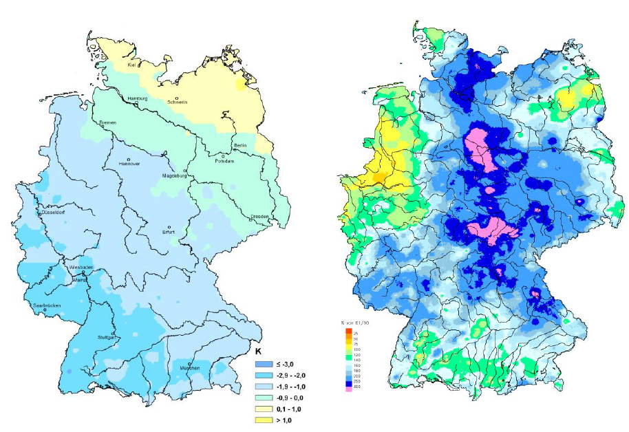
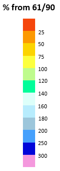
Figure 3.1: Left: Deviation of air temperature in May 2013 from the 1981-2010 average. Right: Precipitation height in May 2013 as a percentage of the 1961-1990 average. Source: (1)
The left chart shows that in May 2013 the southwest was more than 2 K colder. There was a large section of Germany, running from the northwest to the southeast, which was over 1 K below the 1981-2010 average.
The right chart shows precipitation values of double the average (relative to 1961-1990) in May 2013, with some exceptions in the northwest, northeast and some parts of the south. In a wide band from southern Schleswig-Holstein to northern Bavaria the values reached 250% to more than 300% of the monthly average.
The significance of extreme soil moisture at the end of May 2013
Due to the heavy precipitation at the end of May the soil was saturated with water. The recorded soil moisture values were the highest since measurements were begun in 1962. They correspond to the dark blue areas in the following figure, and these areas would also become the flood regions later.
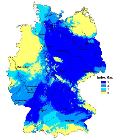
Figure 3.2: Extreme values of soil moisture on 31 May 2013, compared to the 31 May average from 1962 to 2012. Source: (1)
0: no previous records were surpassed
1: third highest recorded value of soil moisture is surpassed
2: second highest recorded value of soil moisture is surpassed
3: highest recorded value of soil moisture is surpassed, new absolute maximum
Figure 3.3: Flooded fields. Potato field on the left, sugar beet field on the right. Source: ZAMG Braunschweig (DWD)
The Moderate Resolution Imaging Spectroradiometer (MODIS) on NASA's Terra satellite observed flooding in central and eastern Germany on 5 May 2013 (before the flood) and on 6 June 2013 (during the flood). On 6 June the Elbe river reached 8.7 meters, while its norm is only 2 meters.
These false-color images use a combination of visible and infrared light to make it easier to distinguish water and land. River water appears dark blue to black and vegetation is bright green. These images are used in situations like floods or forest fires because of their sharp contrast.
Images like these are also available from the new Suomi-NPP satellite and the VIIRS instrument.
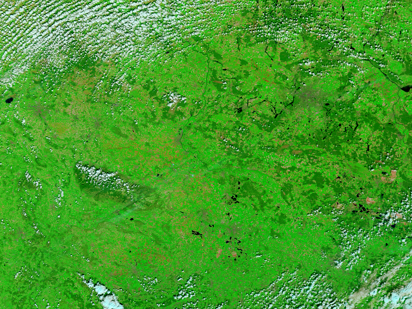
Figure 3.4: 5 May 2013. An image from NASA's Terra satellite with the MODIS instrument, showing the Elbe catchment area. Source:
http://earthobservatory.nasa.gov/NaturalHazards/view.php?id=81287
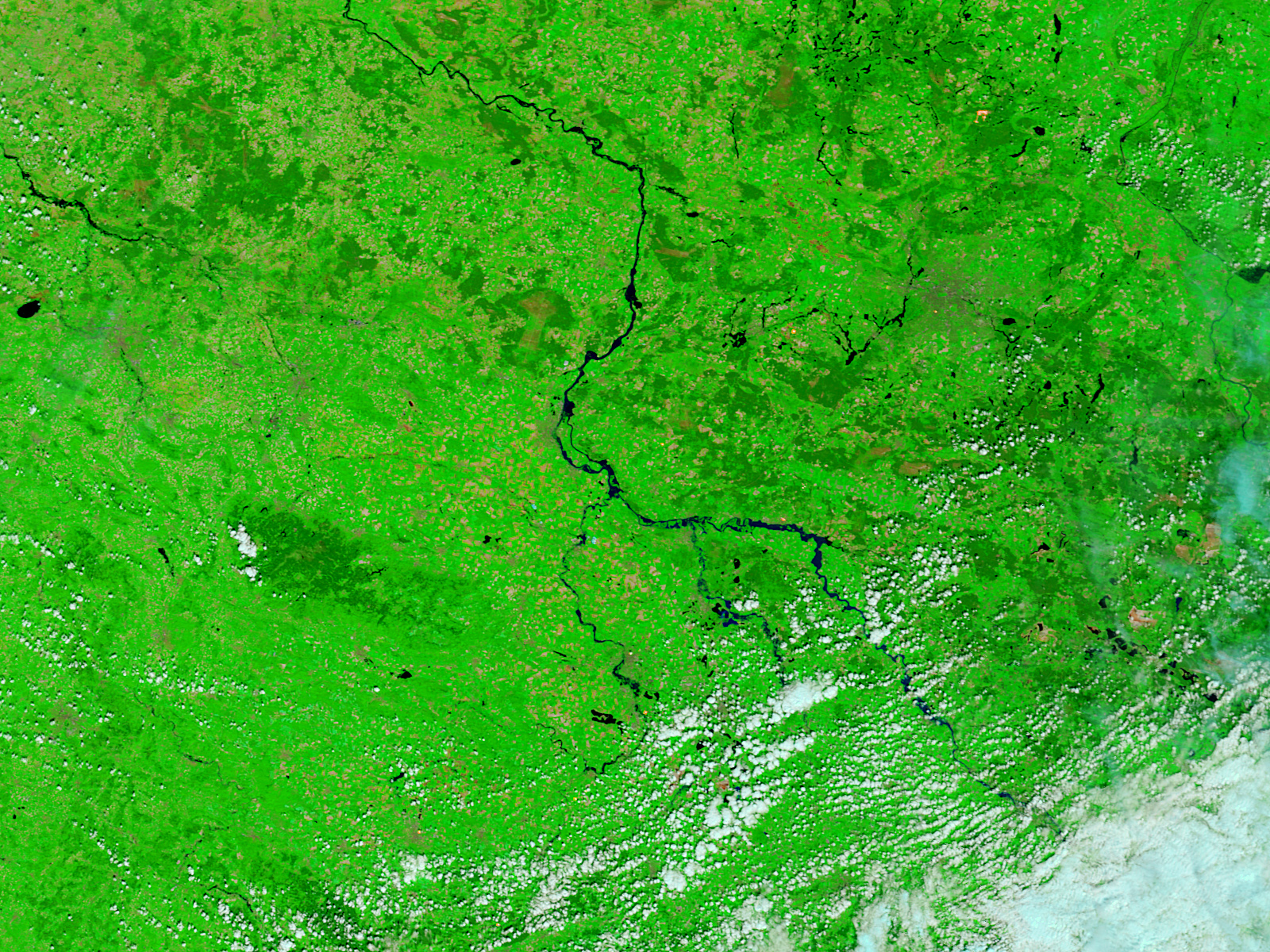
Figure 3.5: 5 June 2013. An image from NASA's Terra satellite with the MODIS instrument, showing the Elbe catchment area. Source:
http://earthobservatory.nasa.gov/NaturalHazards/view.php?id=81287
The influence of snow cover
The analysis of snow cover's influence on the flood will focus on the period with the most precipitation, the days from 26 May to 2 June 2013. Only the Alps had appreciable amounts of snow at this time.
Fig. 3.6 depicts snow water equivalent, with the values in Austria and Switzerland reaching 400 mm and more. Analysis of snow cover's effects on the flood is only necessary in the Danube drainage basin. The calculations come from the SNOW model from Deutscher Wetterdienst. You will find more information here:
http://www.dwd.de/EN/specialusers/water_management/water_management_node.html
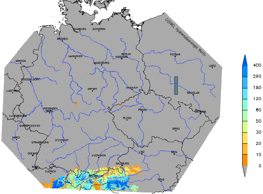
Figure 3.6: The SNOW4 model depicts the snow water equivalent (in mm) of the snow cover on 26 May 2013. Source: (1)
Precipitation, which the snow cover will not hold back, combines with snowmelt and intensifies the flood.
This process was at its strongest on 28 May. The difference between runoff water and precipitation in this area reached 415 billion liters. Fig. 3.7 shows positive values everywhere in the Alps within the covered region.

Figure 3.7: Difference between total runoff and precipitation, 28 May 2013, in the catchment area of the Danube. Source: (1)
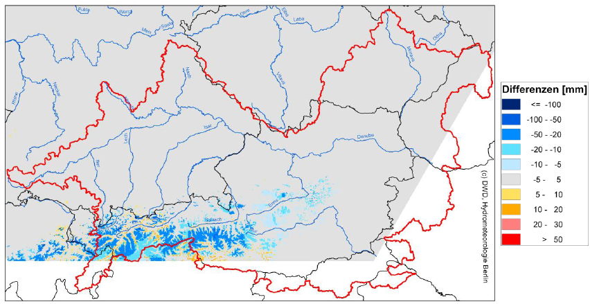
Figure 3.8: Difference between total runoff water and precipitation, 31 May 2013, in the catchment area of the Danube. Source: (1)
If precipitation occurs in the form of snow or rainfall is retained within the snow cover, the runoff is reduced. This process saw its maximum on 31 May, when no snowmelt occurred (see Fig. 3.8). In the catchment area of the Danube 187 billion liters of water were retained in the snow cover.
In summary, snowmelt increased the total runoff by approximately 5%, which means the snow cover played a small part in this flood event.
Summary for the June 2013 flood:
- The soil was saturated in most parts of Germany and could not absorb more water.
- Runoff caused by melting snow was only important near the Alps.
- The snow cover had a small contributing role on the flood.
- The snow cover would have played a more significant part if the event took place during the winter.