Chapter IV: The Tear-Off Stage
The Tear-Off Stage
During the tear-off stage, the upper-level pressure minimum moves away from the band of westerlies. The amplitude of the Rossby wave increases while at the same time the tops of the high-pressure ridges on both sides of the trough converge (see red W in Figure 2). As a consequence, the low-pressure bridge connecting the upper-level pressure minimum to the main pressure minimum gets narrower and narrower. Depending on the motion of the upper-level low, the low-pressure trough tilts either forward or backward. This is the beginning of the cut-off stage (see Figure 1).
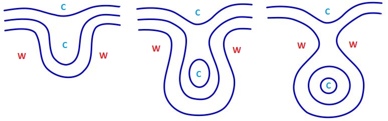
Figure 1: Schematic of the tear-off process from left to right. Blue lines represent the geopotential height at around 500 hPa, red W indicates warm air and blue C cold polar air masses.
The SEVIRI water vapor image loop in Figure 2 shows the whole formation process: the deepening trough, the tear-off and cut-off stages until the ULL has reached its final evolution stage as a drop of cold air south of the polar front. In this winter case example, the cut-off low is located far in the south. Notice the strong gradient of the 500 hPa geopotential lines at the southern tip of the trough which becomes less pronounced as soon as the cold core forms. In the final stage the ULL shows a regular pressure gradient pattern around its core.
Figure 2: WV loop from 21 February 2021 at 00 UTC to 24 February 2021 at 00 UTC. The 500 hPa geopotential height is depicted in cyan isolines.
Let's have a look at the NWP parameters that best characterize the tear-off stage.
Temperature:
The polar air mass inside the core of the upper-level low is much colder than the air surrounding the cold core, and the tropopause is lowered above the core. This can best be seen in a vertical cross section trough the center of the ULL.

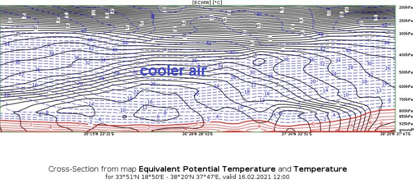
Figure 3: 16 February, 2021 at 12:00 UTC. Above: Position of the vertical cross section through the core of an ULL in the tear-off stage (orientation west to east). Below: Temperature (dotted blue lines) and equivalent potential temperature (black lines).
The temperature contrast between the center of the tear-off low and the surrounding warmer air masses is usually quite strong and is only marginally diminished by adiabatic processes that result from subsidence as long as the pressure minimum of the tear-off low continues to decrease.
Potential Vorticity (PV):
At the location of the ULL the height of the tropopause exhibits a minimum which is seen in the local PV values (see Figure 4). Descending air masses from higher levels create a dry spot that can be seen in water vapor imagery (black circular spot) and in the Airmass RGB (red circular area). Their water vapor signature is most distinct, especially in the phase when the upper-level pressure minimum deepens (i.e., during the tear-off stage).
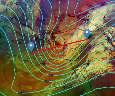
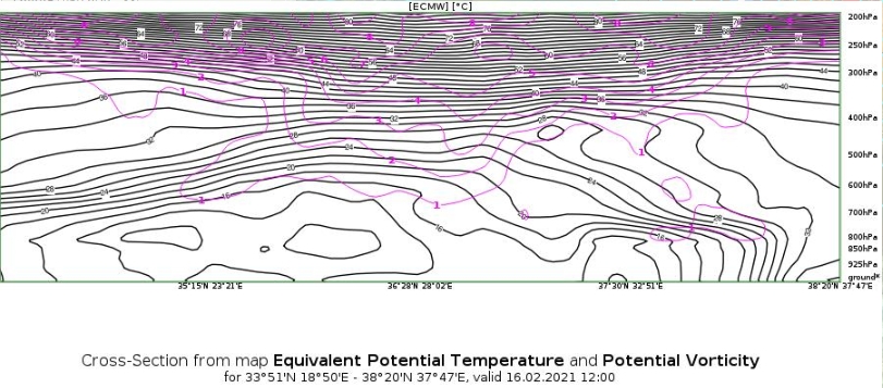
Figure 4: 16 February, 2021 at 12:00 UTC. Above: Position of the vertical cross section though the core of an ULL in the tear-off stage (orientation west to east). Below: Potential Vorticity (magenta lines) and equivalent potential temperature (black lines).
The Jet:
During the tear-off stage, the highest wind speeds within the jet stream are found either on one or both sides of the elongated trough. When an upper-level low forms, the wind speed maximum is rarely found at the southern tip of the trough where the curvature is strongest.
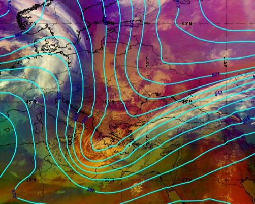
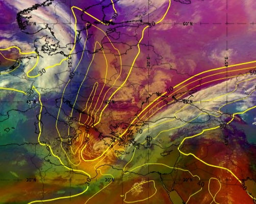
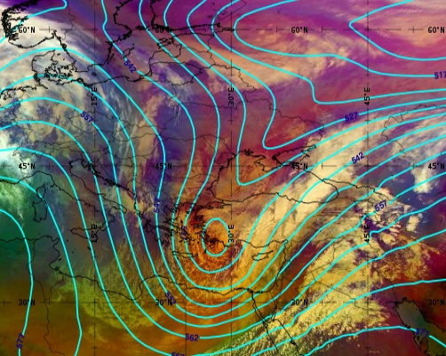
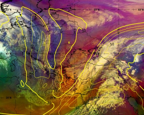
Figure 5: Tear-off stage on 15 and 16 February 2021 at 12:00 UTC. Left: Geopotential height at 500 hPa (cyan). Right: Isotachs at 300 hPa (yellow).
Why Don't Jet Streaks Like Strong Curvature?
Let us first look at the dominant forces that act within a jet streak, or more generally on every air parcel that is carried along with the jet stream in the upper troposphere.
In principle, two forces act on the wind at jet level (i.e., around 300 hPa): the Coriolis force, which is a pseudo force since its strength depends on wind speed, and the pressure gradient force, which acts on any air parcel independent of its speed. In a linear jet and in the absence of friction, both forces compensate for each other. This equilibrium is called the geostrophic equilibrium and hence the wind is called the geostrophic wind (see Figure 6).
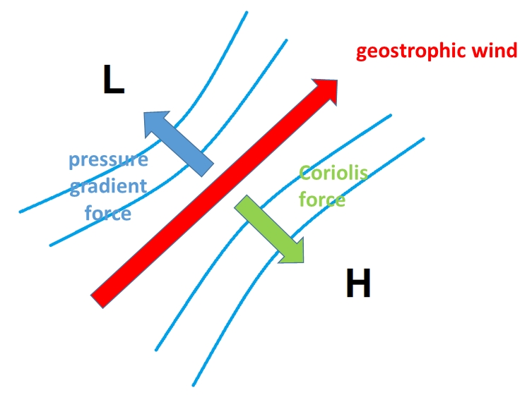
Figure 6: Schematic illustrating the two forces acting on a linear jet wind in the northern hemisphere.
This equilibrium of interacting forces is true for a linear jet. In the case of a curved jet, a second pseudo force enters into the equation: the centrifugal force, which again is dependent on wind speed and hence a pseudo force. The resulting equilibrium between these three forces is called the gradient wind (see Figure 7).
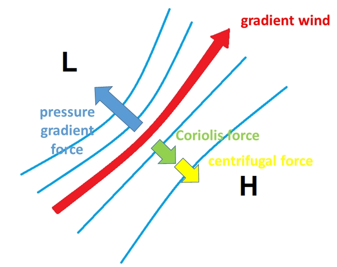
Figure 7: Schematic illustrating the three forces acting on a curved jet stream in the northern hemisphere.
When curvature increases in some parts of the flow around the tear-off low, the wind speed has to decelerate so that both, the Coriolis and centrifugal forces both of which are pseudo forces that depend on wind speed can be compensated by pressure gradient forces (see Figure 7). Therefore, whenever curvature increases while pressure gradient forces stay the same along the jet's trajectory, wind speed deceleration is necessary. This is a common situation for a cut-off low during the tear-off process and this is also why we usually observe jet streaks on both sides of a trough and not at its southern tip where curvature is strongest.
As shown in Figure 8, the wind speed of the jet stream clearly decelerates when the airflow turns around the sharp edge of the upper-level trough. The pressure gradient force at the southern tip of the ULL, where curvature is strongest, does not increase in order to compensate for the Coriolis and centrifugal forces. As a result, the wind speed has to decrease to make it round the "corner".
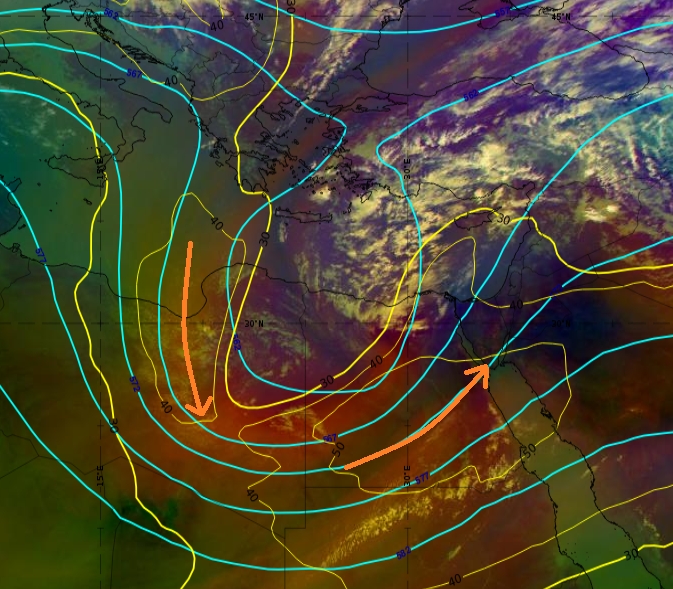
Figure 8: Airmass RGB from 3 February 2021 at 12:00 UTC. Isotachs at 300 hPa are depicted in yellow and the geopotential height at 500 hPa in cyan. The orange arrows mark the position of the jet streaks.
Note:
Whether a jet streak is split into two branches or not when circling a trough or an upper-level low mainly depends on the interplay of pressure gradient and curvature. Upper-level lows with a uniform pressure gradient tend to have a continuous wind speed along the jet's path while troughs with a sharp southern edge tend to show split jet streaks on each side of the trough.
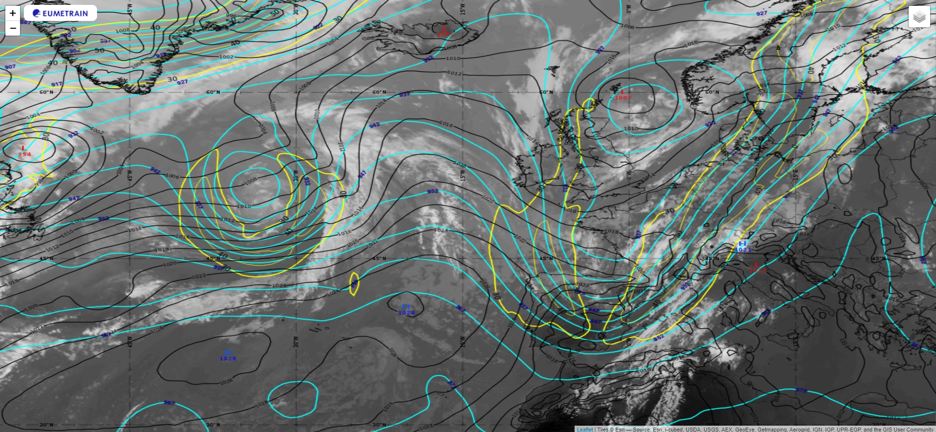
Figure 9: IR 10.8 μm from 7 July 2021 at 18:00 UTC. Isotachs at 300 hPa in yellow, geopotential height at 300 hPa in blue and mean surface level pressure in black.
The example above (see Figure 9) shows a pronounced trough over western Europe and an upper-level low over the Atlantic. The weather situation can be classified as low index circulation and both features are located amid warm air far south of the polar front: a meteorological condition that is typical for northern hemispheric summer.
While pressure gradient forces increase south of the ULL (feature on the left) and thus compensate for the Coriolis and centrifugal forces, the pressure gradient merely stays constant for the airflow contouring the southern tip of the trough (feature on the right). This results in a constant wind speed around the ULL, while the trough has a wind speed minimum near the place of strongest curvature.