Chapter III: Side by side comparison of a Norwegian Cyclone (9 - 13 March 2019) and a Shapiro-Keyser Cyclone (14 - 17 March 2019)
Table of Contents
- Chapter III: Side by side comparison of a Norwegian Cyclone and a Shapiro-Keyser Cyclone
- Side by side comparison of a Norwegian Cyclone and a Shapiro-Keyser Cyclone
Side by side comparison of a Norwegian Cyclone (9 - 13 March 2019) and a Shapiro-Keyser Cyclone (14 - 17 March 2019)
Let us make another side by side comparison of the two cyclone types, but this time with example cases. For both cyclones, we will follow the five previously defined development stages and look closely at NWP parameters.
The loops below show a cyclogenesis of the Norwegian type (left) and a cyclogenesis of the Shapiro-Keyser type (right).
Figure 1:
Left: Life cycle of a Norwegian cyclone (9 March 2019, 21:00 UTC to 12 March 2019, 06:00 UTC)
Right: Life cycle of a Shapiro-Keyser cyclone (15 March 2019, 18:00 UTC to 17 March 2019, 18:00 UTC)
A) Initial stage
Both cyclone examples start from the same preconditions: a horizontal temperature gradient in an undisturbed flow along a baroclinic boundary.
|
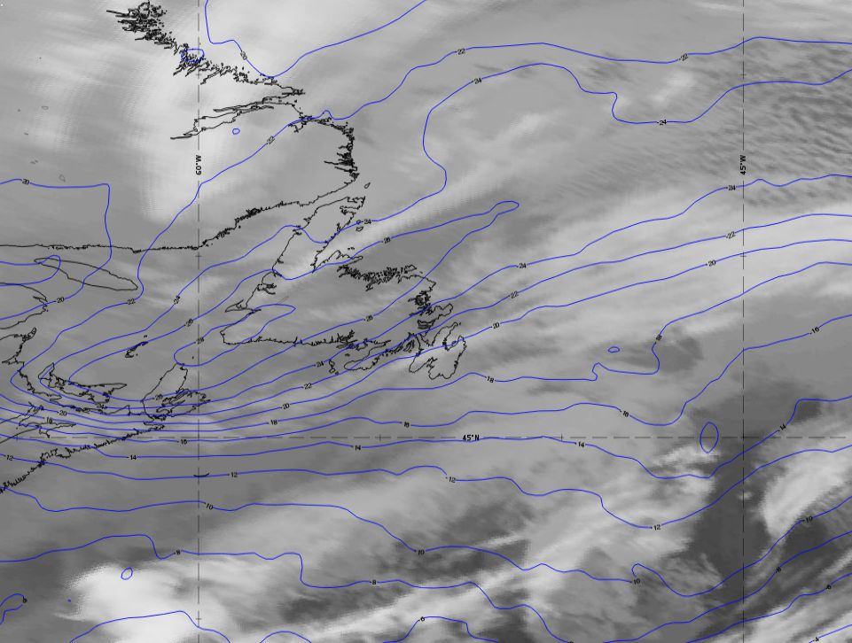
Norwegian Cyclone The initial stage is characterized by a zonal temperature gradient with warm temperatures to the south and cold temperatures in the north. |
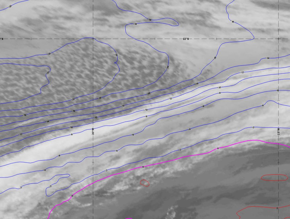
Shapiro-Keyser Cyclone (S-K) The starting point for this S-K cyclone is a well-defined stationary frontal zone that separates cold air in the north from warmer air masses in the south. |
|
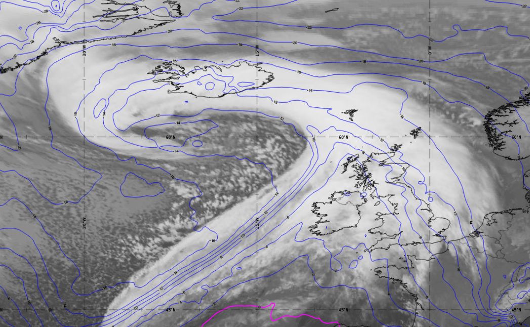
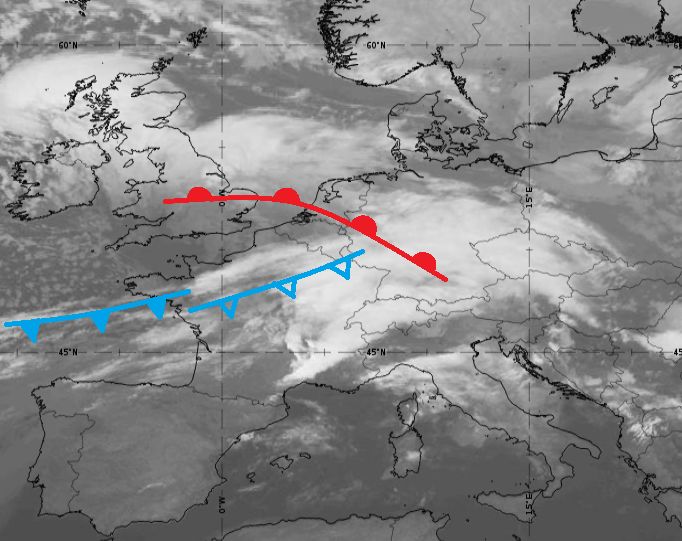
Figure 1a: SEVIRI IR10.8 μm image. Blue lines indicate temperature at 700 hPa. In the IR-imagery, a west to east oriented baroclinic boundary (i.e., stationary front) can be discerned. |
Figure 1b: SEVIRI IR10.8 μm image. Blue/magenta lines indicate temperature at 700 hPa. In the IR-imagery, a west to east oriented baroclinic boundary (i.e., stationary front) can be discerned. |
|
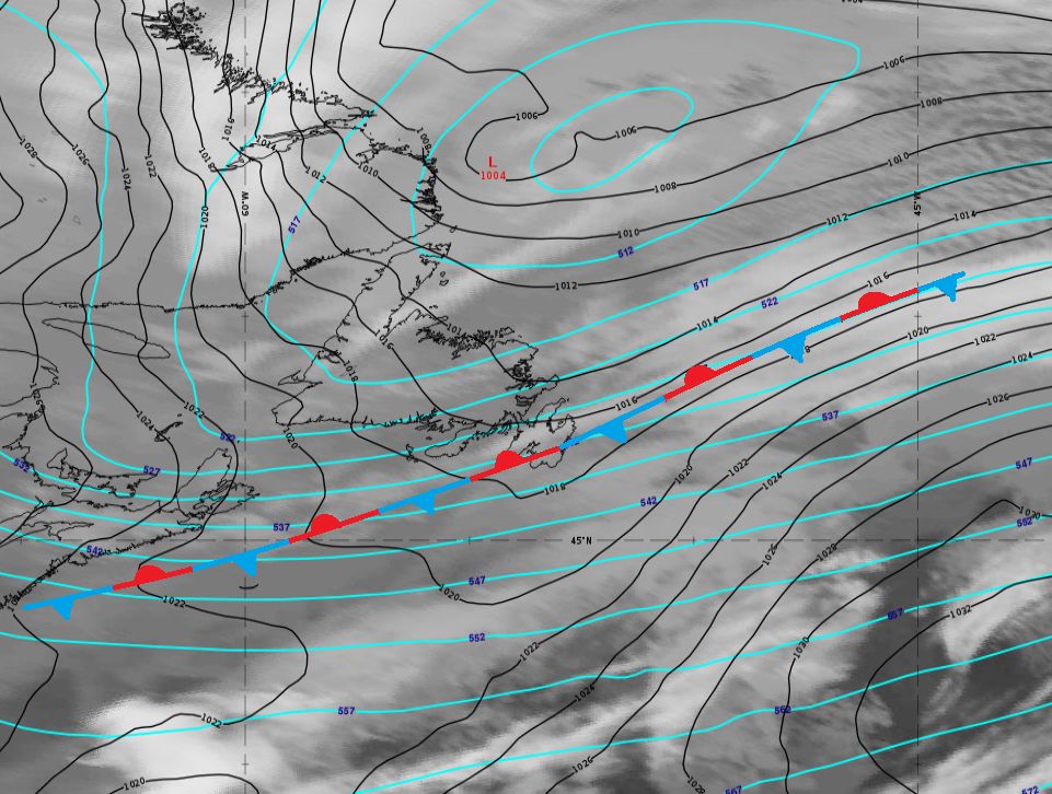
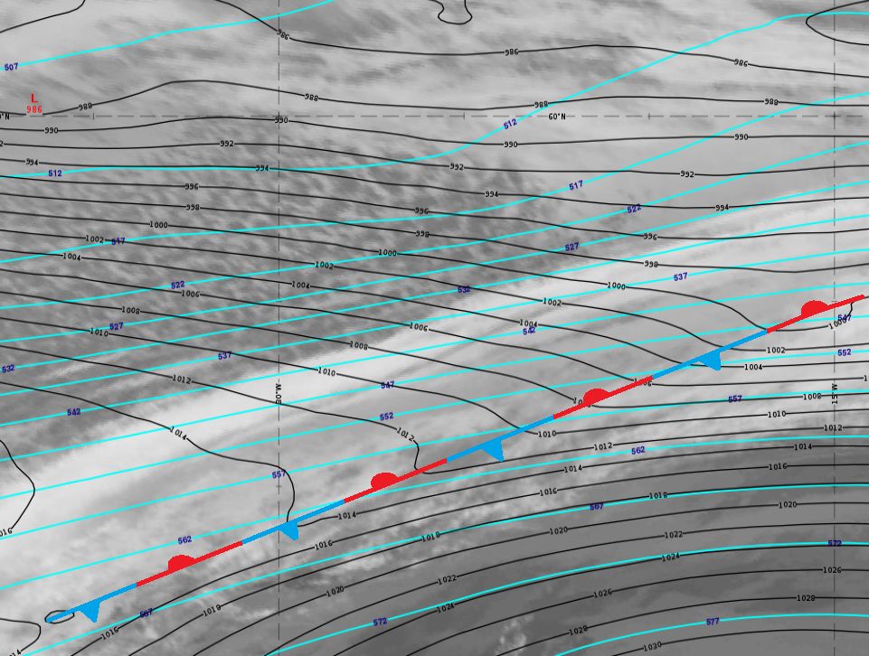
Figure 2a: SEVIRI IR10.8 μm image. Mean sea level pressure (black) and geopotential height at 500 hPa (cyan). A jet with its maximum around 300 hPa accompanies the zonal temperature gradient. |
Figure 2b: SEVIRI IR10.8 μm image. Mean sea level pressure (black) and geopotential height at 500 hPa (cyan). A jet with its maximum around 300 hPa accompanies the zonal temperature gradient. |
|
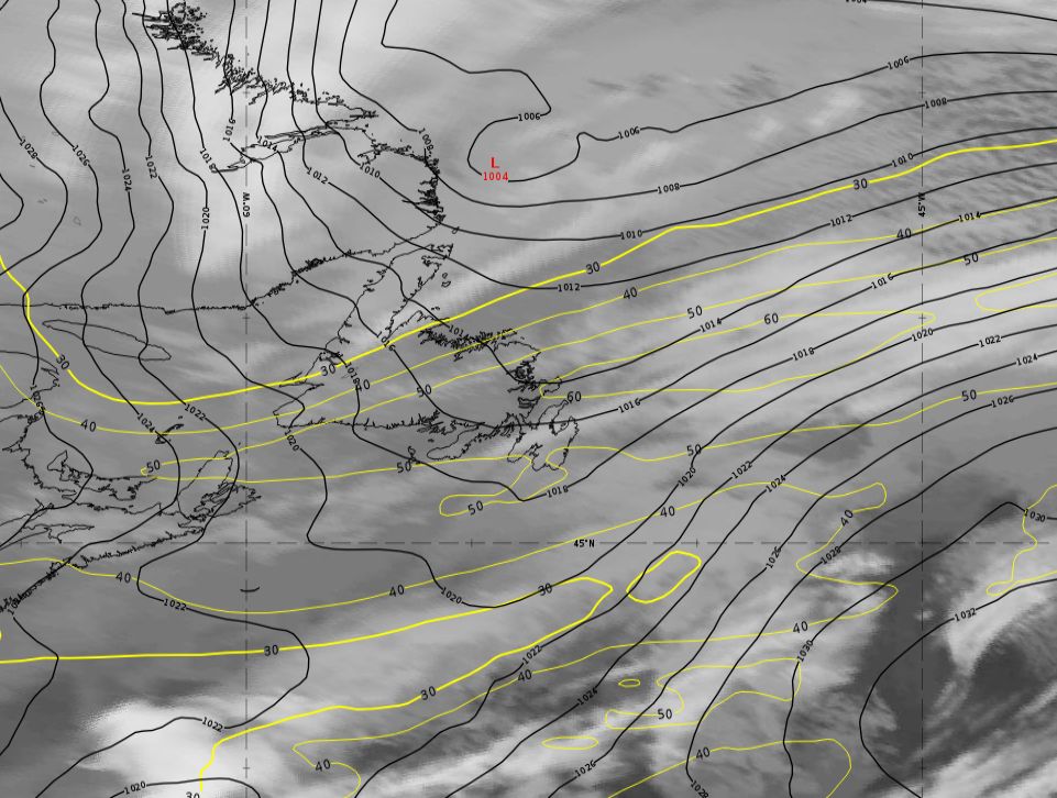
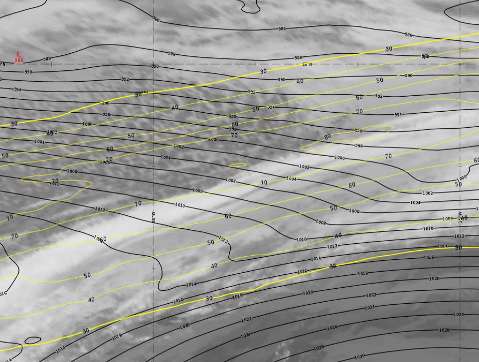
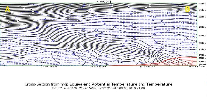
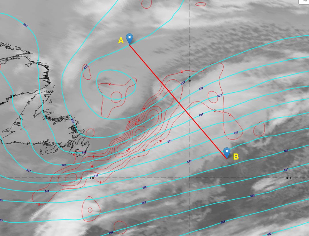
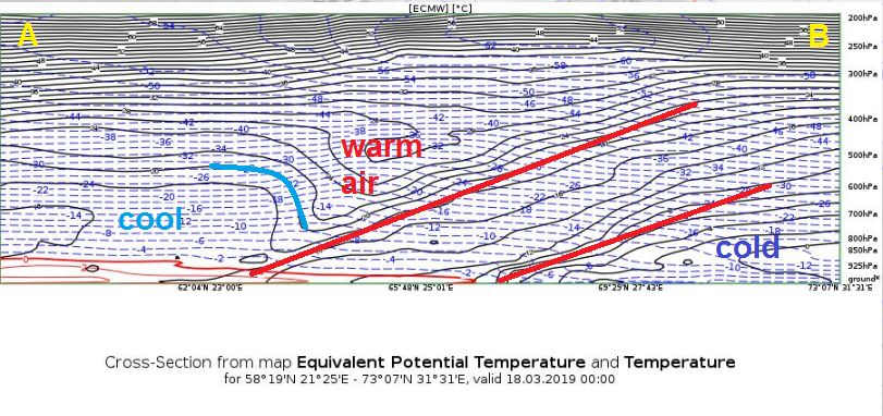
Figure 3a: SEVIRI IR10.8 μm image. Mean sea level pressure (black) and isotachs at 300 hPa (yellow). Vertical cross section: A cross section through the baroclinic boundary shows a pronounced temperature gradient with a strong inclination of the isolines of equivalent potential temperature. This is a clear indication of a slowly moving or stationary front. |
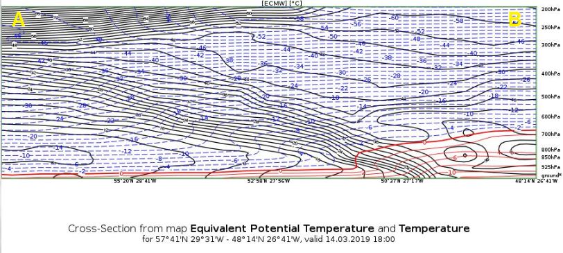
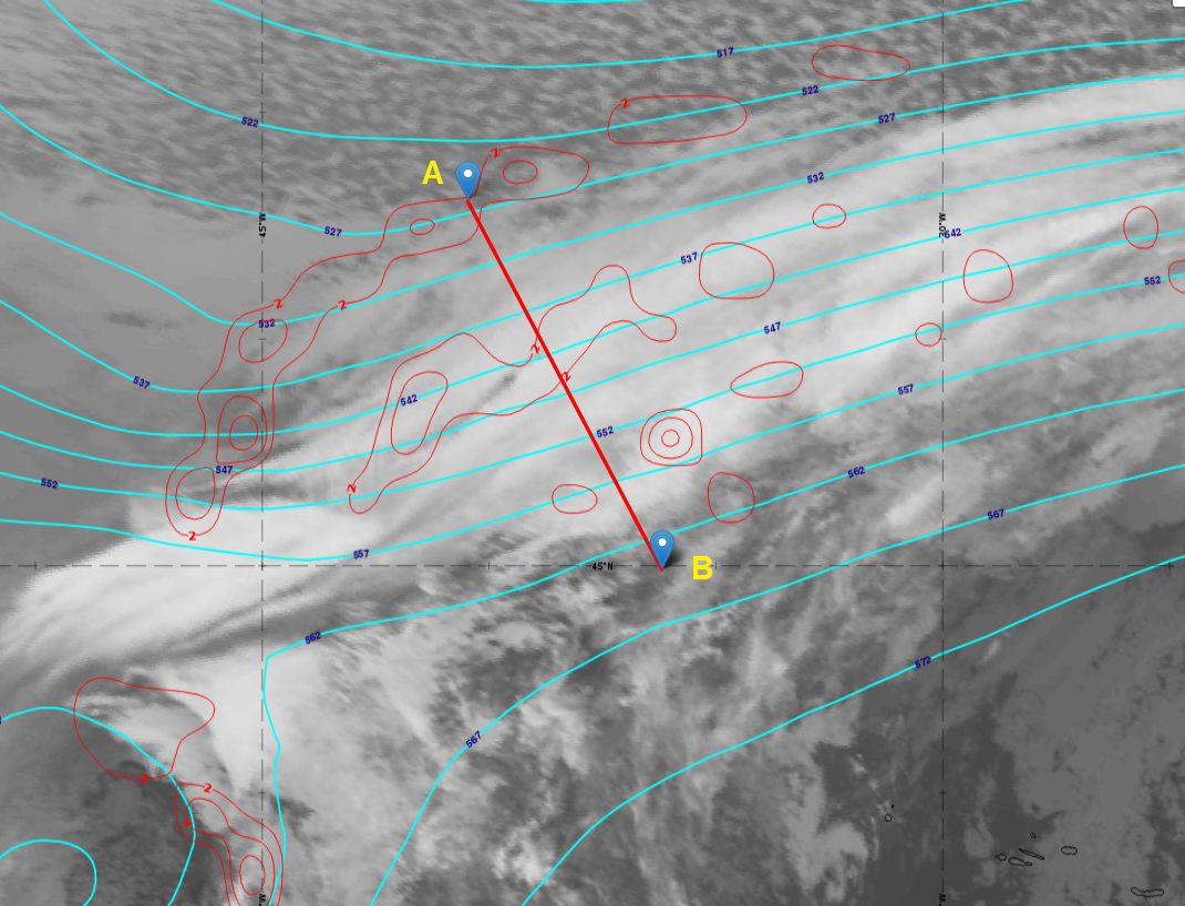
Figure 3b: SEVIRI IR10.8 μm image. Mean sea level pressure (black) and isotachs at 300 hPa (yellow). Vertical cross section: A cross section through the baroclinic boundary shows a pronounced temperature gradient with a strong inclination of the isolines of equivalent potential temperature. This is a clear indication of a slowly moving or stationary front. |
|
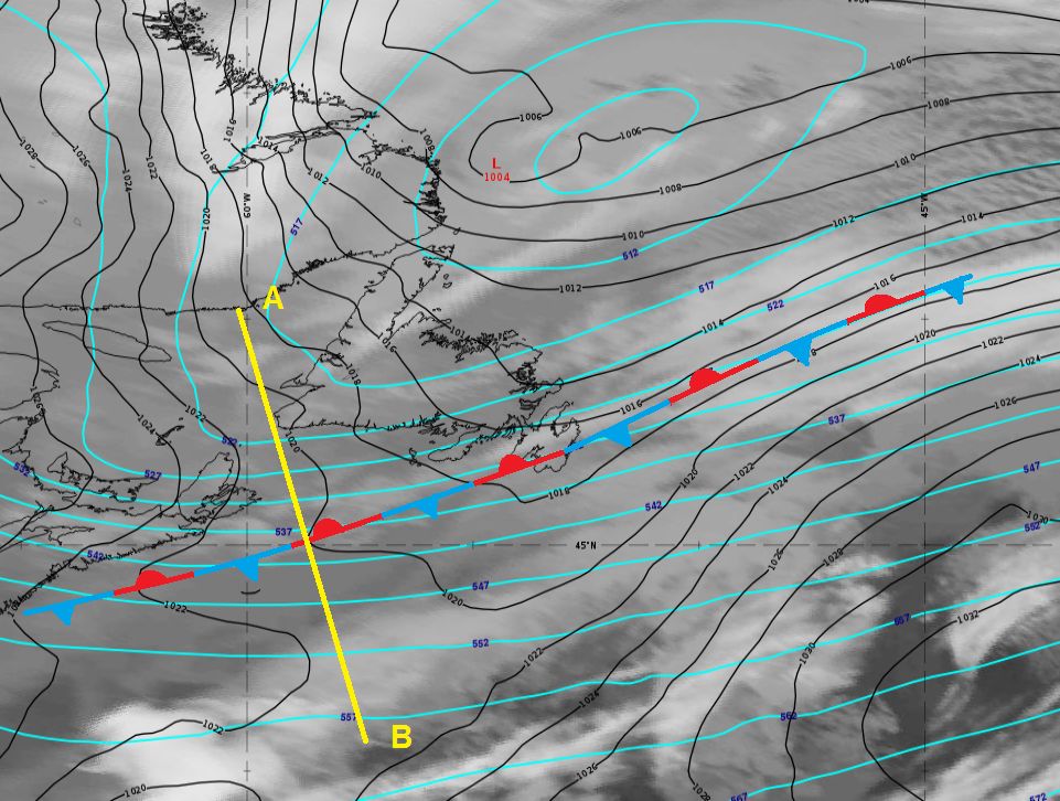
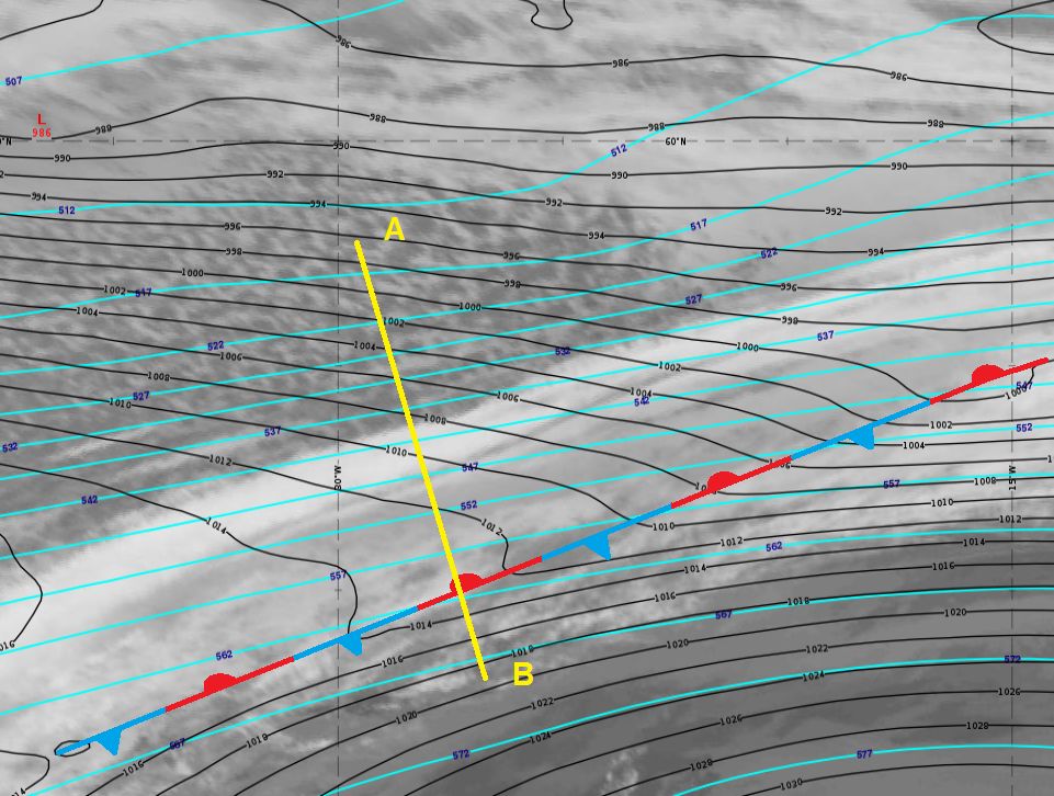
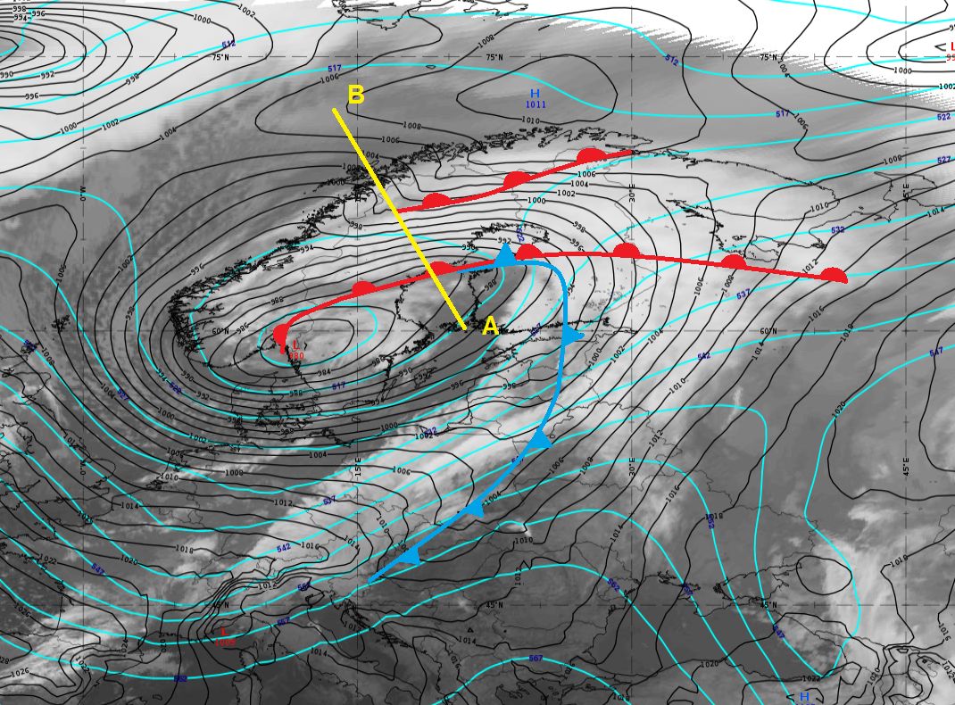
Figure 4a: SEVIRI IR10.8 μm image with a yellow line indicating the position of the vertical cross section. Mean sea level pressure (black) and geopotential height at 500 hPa (cyan). |
Figure 4b: SEVIRI IR10.8 μm image with a yellow line indicating the position of the vertical cross section. Mean sea level pressure (black) and geopotential height at 500 hPa (cyan). |
|
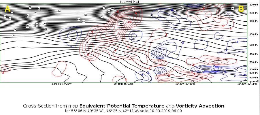
Figure 5a:1 Cross section (north to south) from the ECMWF model. |
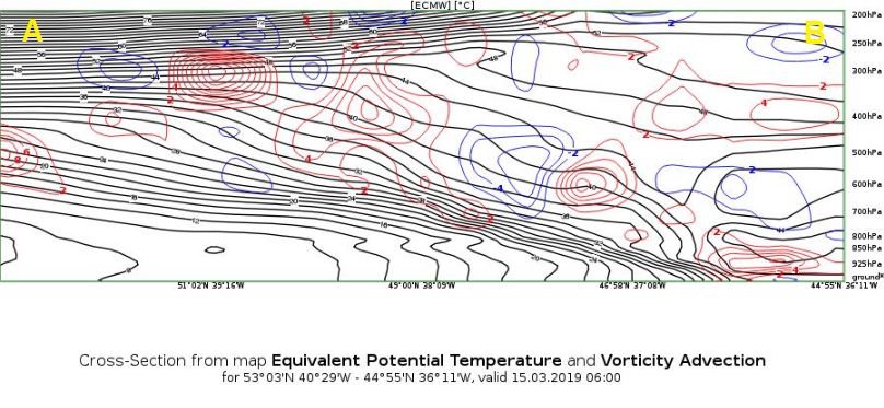
Figure 5b: Cross section (north to south) from the ECMWF model. |
Quiz:
Are there early indications as to whether the developing cyclone is of the Norwegian or S-K type at this initial stage? Select only one answer!
B) Developing wave
The development of the surface low is triggered by the upper-level dynamics. The curvature of the geostrophic flow produces areas of divergence and convergence that influence the vertical motion of the air at lower levels.
There are no major differences between the Norwegian and the Shapiro-Keyser cyclone model types in the early development phase, except for the upper-level background flow.
|
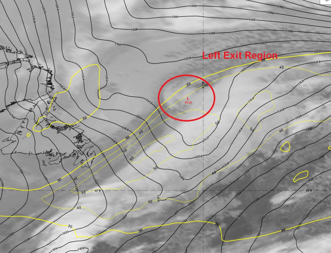
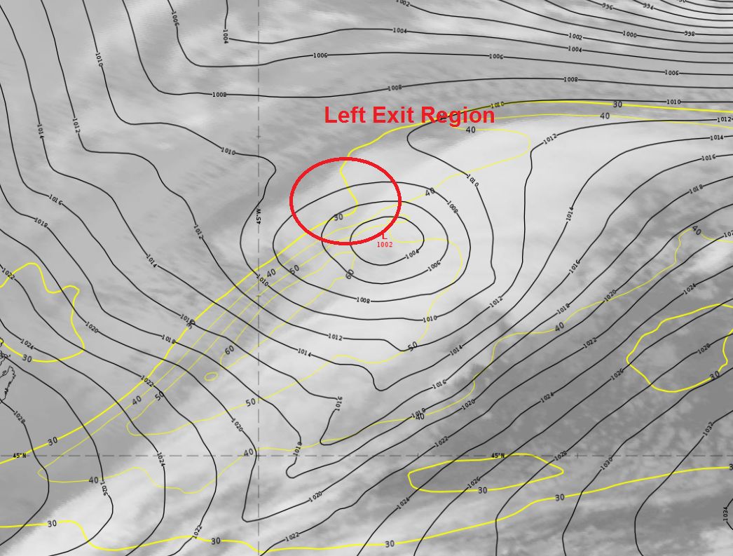
Norwegian Cyclone During the next stage, a surface low starts to develop below the left-exit quadrant of the jet. |
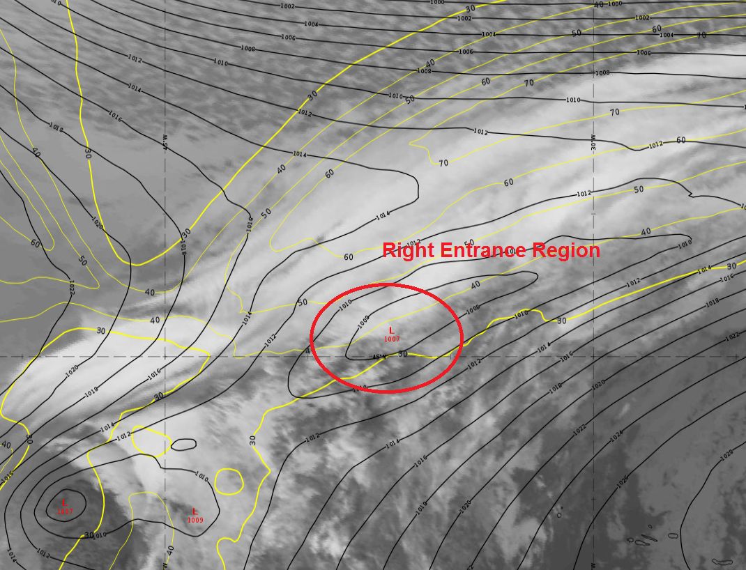
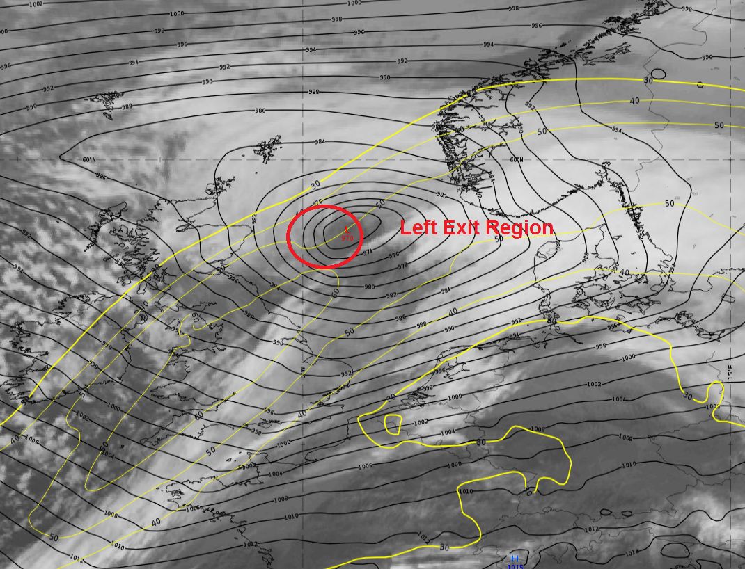
Shapiro-Keyser Cyclone (S-K) In this example, the surface low of the S-K cyclone starts developing at the ascending branch of the jet cross circulation below the right-entrance quadrant of the jet. However, it can also develop in the left-exit quadrant of the jet. During a later development stage, the center moves towards the left-exit quadrant of the jet. |
|
Figure 1a: SEVIRI IR10.8 μm image. Mean sea level pressure (black) and isotachs at 500 hPa (yellow). The vertical axis of the developing cyclone is strongly inclined towards the west (i.e., tilted backwards) and the background flow at 500 hPa is slightly divergent above the surface low. |
Figure 1b: SEVIRI IR10.8 μm image. Mean sea level pressure (black) and isotachs at 300 hPa (yellow). The vertical axis of the developing cyclone is strongly inclined towards the west (i.e., tilted backwards) and the background flow at 500 hPa is slightly convergent above the surface low. |
|
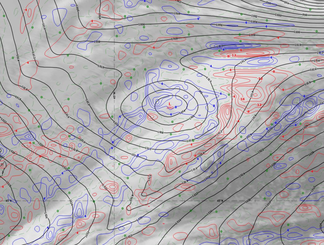
Figure 2a: SEVIRI IR10.8 μm image. Mean sea level pressure (black) and geopotential height at 500 hPa (cyan). The temperature advection field indicates protruding warm and cold air masses and developing fronts. |
Figure 2b: SEVIRI IR10.8 μm image. Mean sea level pressure (black) and geopotential height at 500 hPa (cyan). The temperature advection field indicates protruding warm and cold air masses and developing fronts. |
|
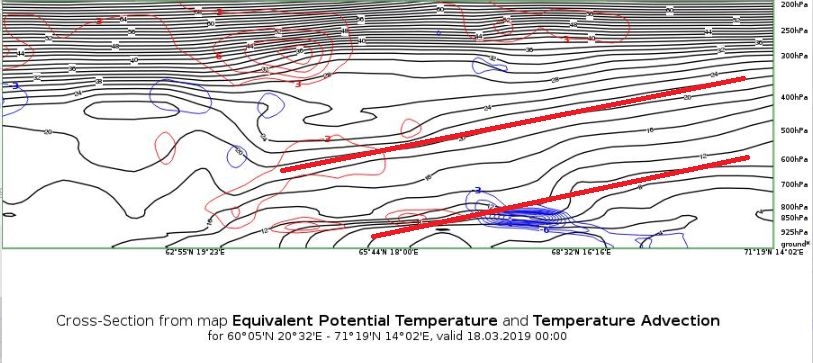
Figure 3a: SEVIRI IR10.8 μm image. Mean sea level pressure and temperature advection at 850 hPa. Vertical cross section: The vertical cross section through the area of the surface low shows increasing positive vorticity advection with height on the leading edge of the shortwave trough. This is a necessary precondition for lifting. |
Figure 3b: SEVIRI IR10.8 μm image. Mean sea level pressure and temperature advection at 850 hPa. Vertical cross section: The vertical cross section through the area of the surface low shows increasing positive vorticity advection with height on the leading edge of the shortwave trough. This is a necessary precondition for lifting. |
|
Figure 4a: SEVIRI IR10.8 μm image with a red line indicating the position of the vertical cross section. Cyan lines show the geopotential height at 500 hPa, red isolines the cyclonic vorticity advection at the same level. |
Figure 4b: SEVIRI IR10.8 μm image with a red line indicating the position of the vertical cross section. Cyan lines show the geopotential height at 500 hPa, red isolines the cyclonic vorticity advection at the same level. |
|
Figure 5a: Cross section (north-west to southeast) from the ECMWF model. |
Figure 5b: Cross section (north-west to southeast) from the ECMWF model. |
Quiz:
What is the most important feature in the developing stage? Select only one answer!
C) Intensification stage
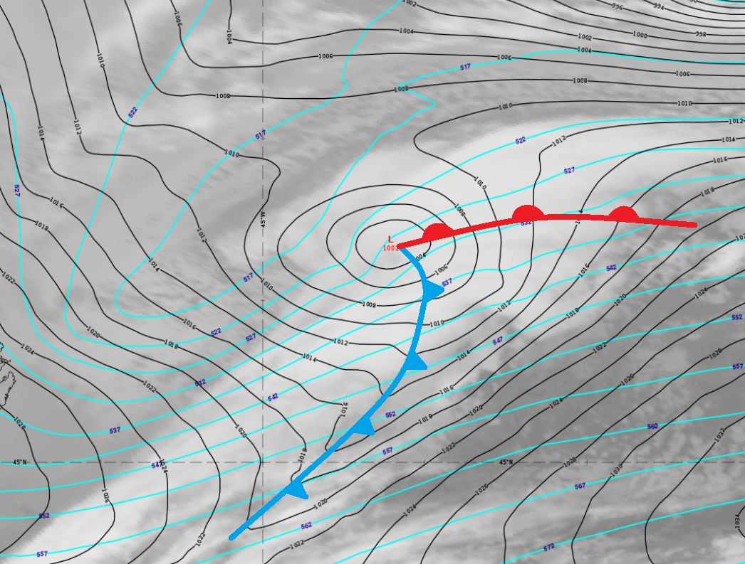
During the intensification stage, the main differences between the Norwegian and the Shapiro-Keyser cyclone models begin to appear. While for the Norwegian cyclone, the warm sector starts to narrow, leaving the cyclone center in cold air, we find the Shapiro-Keyser cyclone center invaded by warm air at lower levels, with a gap opening between the cold and the warm front and the warm front starting to wrap around the pressure minimum.
|
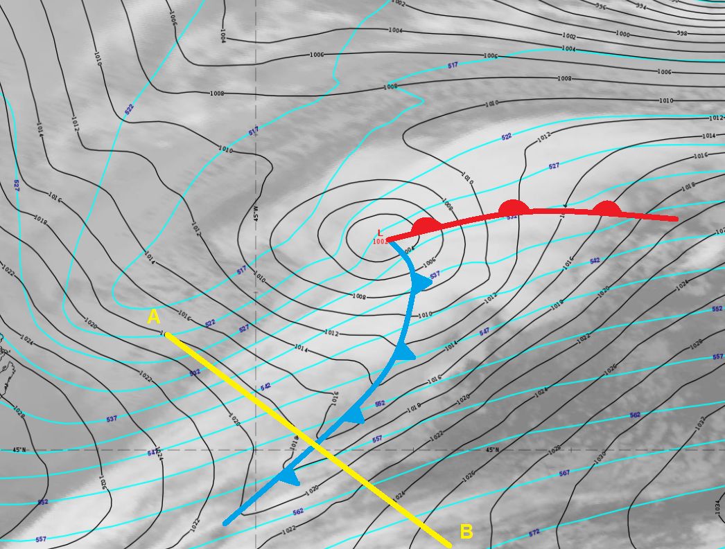
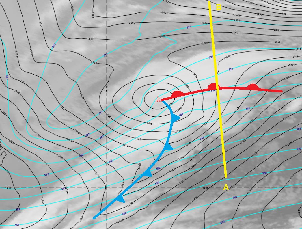
Norwegian Cyclone During the intensification phase, the cold and warm front become stronger and are easily detectable in IR satellite imagery. The vertical axis of the cyclone becomes steeper, the surface pressure decreases rapidly and the pressure gradient increases. The position of the cold front near the ground is indicated by a kink in the surface pressure isolines (black lines). The cold and warm front intersect at an acute angle. |
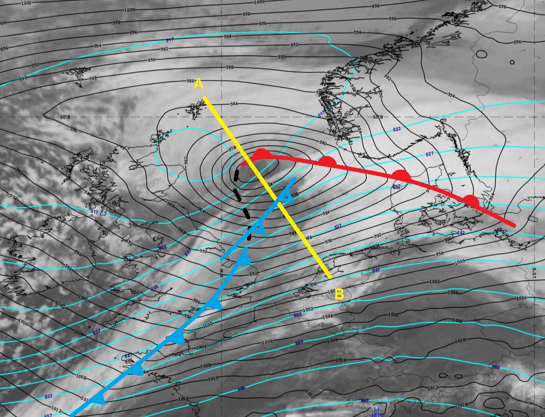
Shapiro-Keyser Cyclone (S-K) During the intensification phase, the center pressure of the S-K cyclone drops rapidly and the upper-level pressure minimum approaches the surface low. The surface cold front detaches from the warm front and the so-called cold frontal fracture (black dotted line) forms. The upper-level cold front remains unaffected by the low-level warm air advance and moves south-eastward. In contrast to the Norwegian model, the surface low remains completely in warm air at lower levels. |
|
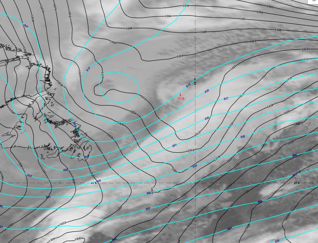
Figure 1a: SEVIRI IR10.8 μm image. Mean sea level pressure (black) and geopotential height at 500 hPa (cyan). The deepening surface low increases the cyclonic circulation and brings more warm air to the north and cold air masses towards the south. Hence, the warm and cold advection become stronger. |
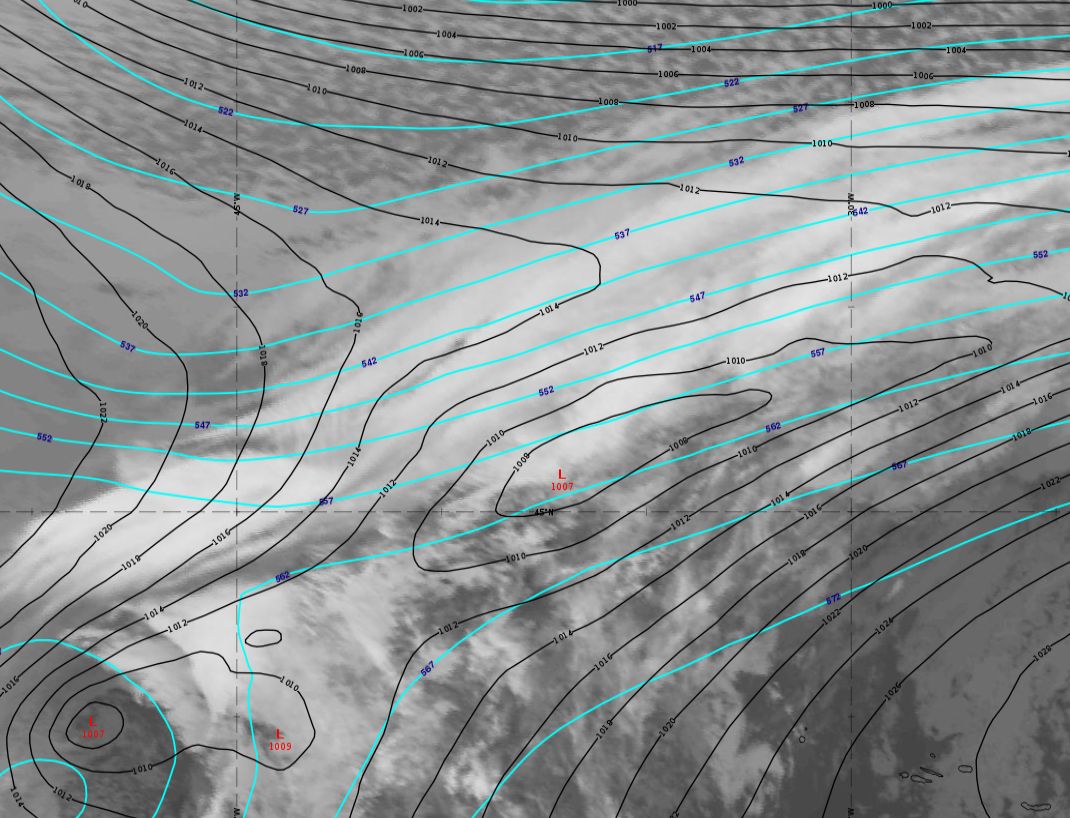
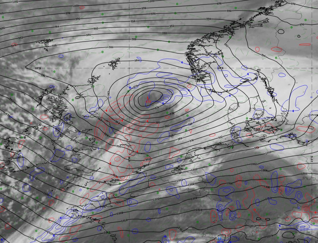
Figure 1b: SEVIRI IR10.8 μm image. Mean sea level pressure (black) and geopotential height at 500 hPa (cyan). Remarkably, and contrary to the Norwegian cyclone type, the temperature field at lower levels shows a pronounced bulge of warm air right at the surface pressure minimum. This is the starting point of the warm seclusion process, where the warm core of the cyclone forms. |
|
Figure 2a: SEVIRI IR10.8 μm image. Temperature advection at 700 hPa. The surface low continues to deepen due to the lifting air that corresponds to the rising branch of the jet cross circulation in the left-exit quadrant of the jet. |
Figure 2b: SEVIRI IR10.8 μm image. Mean sea level pressure and temperature at 850 hPa. As for the Norwegian cyclone, the pressure minimum is located in the left-exit quadrant of the jet. In many cases (but not in this example), there are two branches of the jet and the surface low is located in the left exit region of one branch and simultaneously in the right entrance region of the other. |
|
Figure 3a: SEVIRI IR10.8 μm image. Mean sea level pressure (black) and isotachs at 300 hPa (yellow). Upper-level divergence remains important. |
Figure 3b: SEVIRI IR10.8 μm image. Mean sea level pressure (black) and isotachs at 300 hPa (yellow). Upper-level divergence remains important. |
|
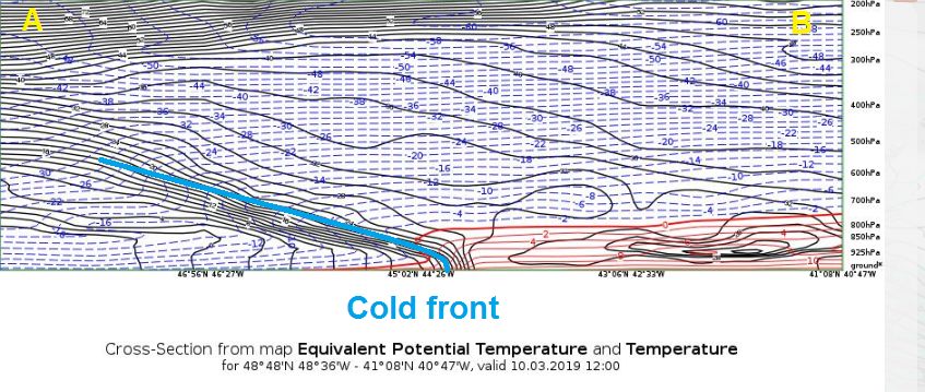
Figure 4a: SEVIRI IR10.8 μm image. Mean sea level pressure (black) and divergence (blue) at 300 hPa. Vertical cross sections: The vertical cross section through the cold front part of the cyclone shows a pronounced temperature gradient with a steeper gradient zone near the ground, which is typical for a cold front (blue line). |
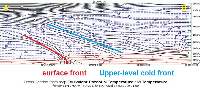
Figure 4b: SEVIRI IR10.8 μm image. Mean sea level pressure (black) and divergence (blue) at 300 hPa. Vertical cross section: The vertical cross section through the warm core of the S-K cyclone shows two frontal zones: a surface front (red) and an upper-level cold front (blue). The surface front has been deformed due to the warm air protrusion. It now delimits the warm core from the cold air to the north. |
|
Figure 5a: SEVIRI IR10.8 μm image with a yellow line indicating the position of the vertical cross section. Cyan lines show the geopotential height at 500 hPa, and black isolines the mean sea level pressure. |
Figure 5b: SEVIRI IR10.8 μm image with a yellow line indicating the position of the vertical cross section. Cyan lines show the geopotential height at 500 hPa, and black isolines the mean sea level pressure. |
|
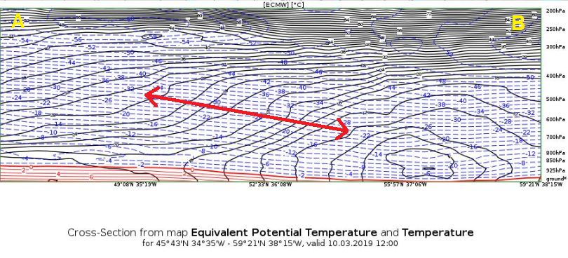
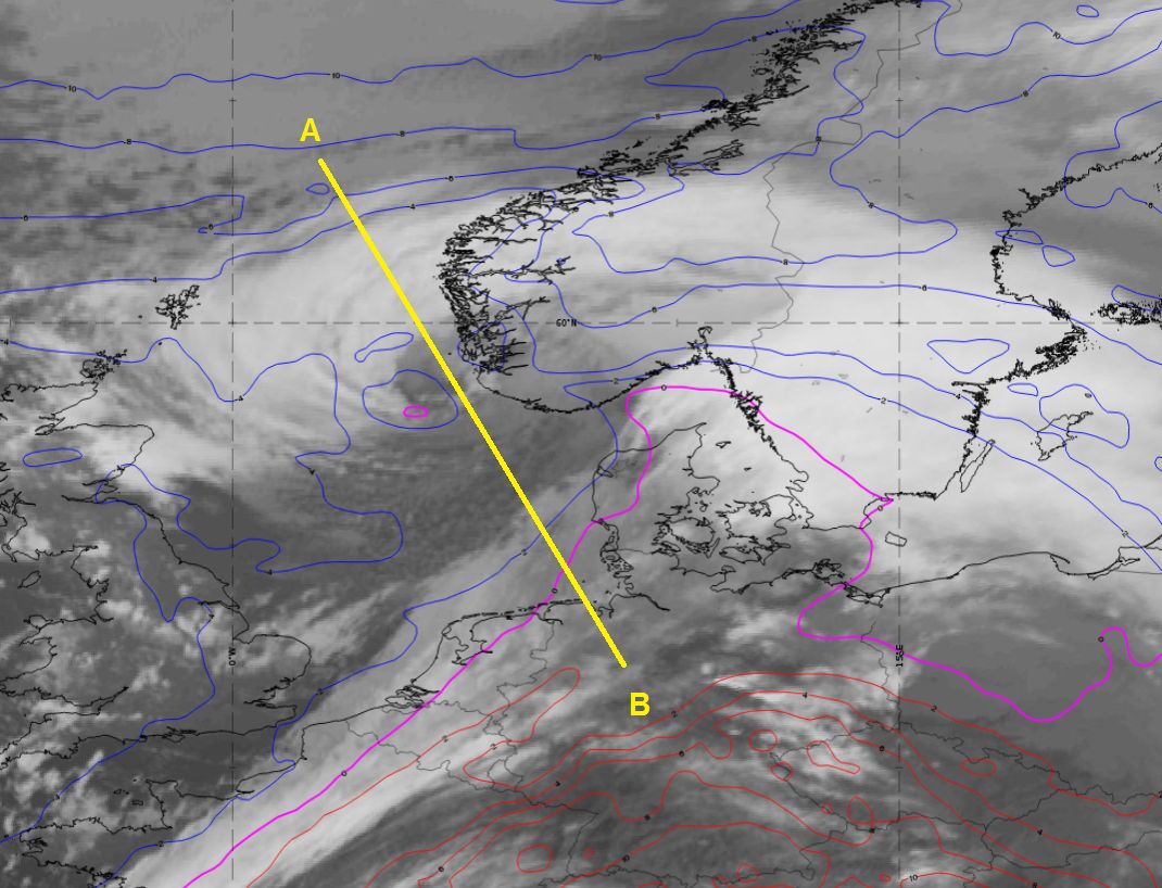
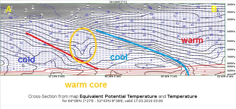
Figure 6a: Cross section (northwest to southeast) from the ECMWF model. In the Norwegian model, the warm front, especially in early stages, does not show such a well-defined temperature gradient as for the cold front; instead it shows a broad transition zone from warm to cold air. In this case, there is no clearly defined surface front. |
Figure 6b: Cross section (northwest to southeast) from the ECMWF model. A closer look at the warm front indicated as “surface front” in Figure 6b reveals that during intensification stage, this frontal zone still shows characteristics of a cold front (though drawn as warm front in Figure 5b), i.e., the steeper part of the frontal zone near the surface and the high temperature gradient. In fact, from the evolution point of view, this is a former cold front that now delimits the recently formed warm air bulge. |
|
Figure 7a: SEVIRI IR10.8 μm image with a yellow line indicating the position of the vertical cross section. Cyan lines show the geopotential height at 500 hPa, and black isolines the mean sea level pressure.
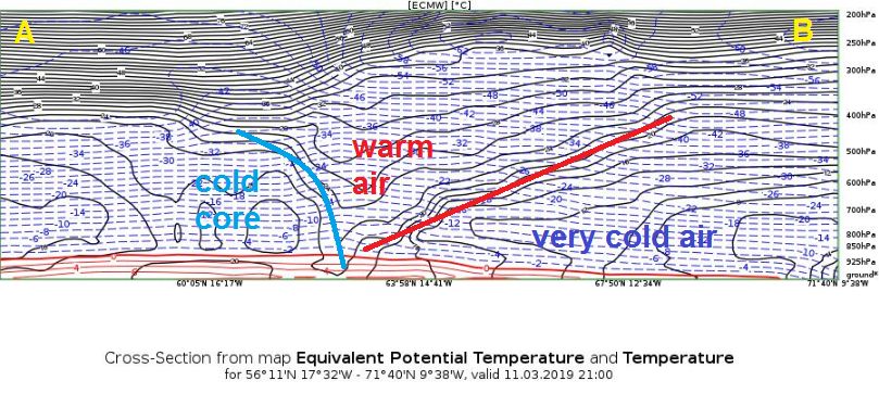
Figure 8a: Cross section (south to north) from the ECMWF model. The red arrow indicates the warm frontal zone. |
Quiz:
What is the main difference during the intensification stage between the Norwegian cyclone and the S-K cyclone? Select only one answer!
D) Maturity stage
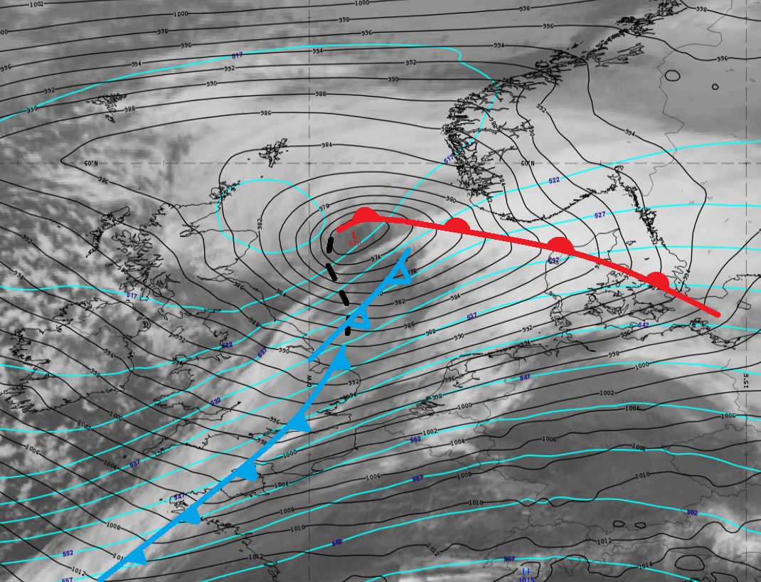
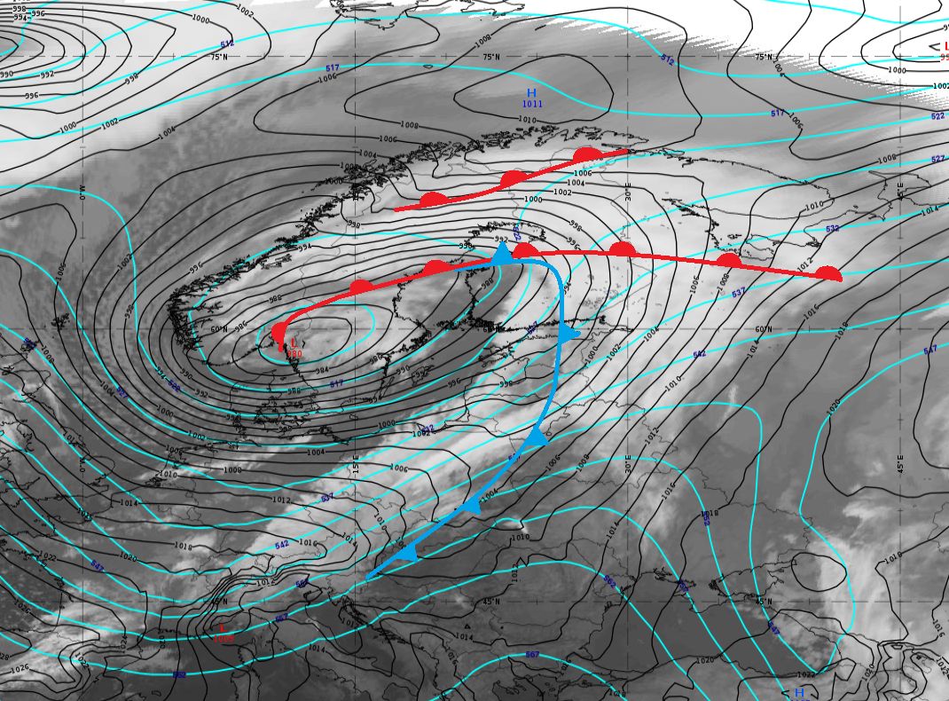
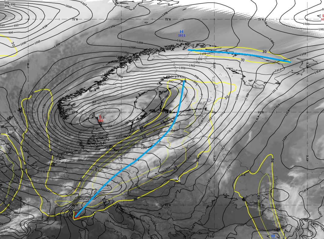
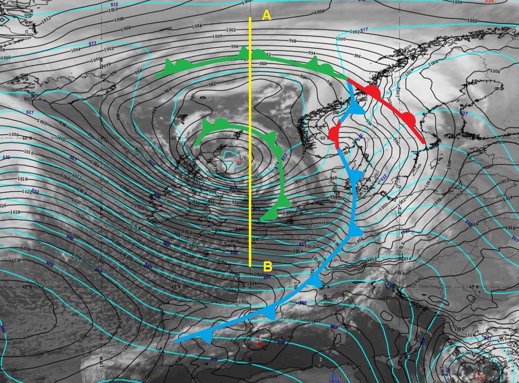
During maturity stage, both cyclone types reveal their major characteristics and differences. For the Norwegian type, the occlusion process starts, i.e., the merging of the warm with the cold front; for the Shapiro-Keyser type, the warm core separates and the typical T-bone structure appears. We observe the formation of a cloud spiral (commonly defined as the occlusion) which is, for S-K cyclones, not the result of the classical occlusion process described by the Norwegian cyclone theory. In fact, it is an air mass boundary that delimits the warm core from surrounding cold air, and which becomes more and more warm-front-like.
|
Norwegian Cyclone The maturity stage of the Norwegian cyclone is characterized by the vertical superposition of the pressure minima of each level. The center pressure at the surface level has reached its minimum value. Near the center of the cyclone, the faster moving cold front catches up with the warm front, forming an occluded front. Inside the occluded front, the warm air from the warm sector is "squeezed" between colder air masses and the air is lifted releasing moisture and latent energy. |
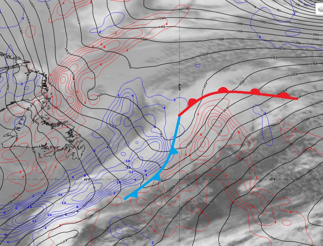
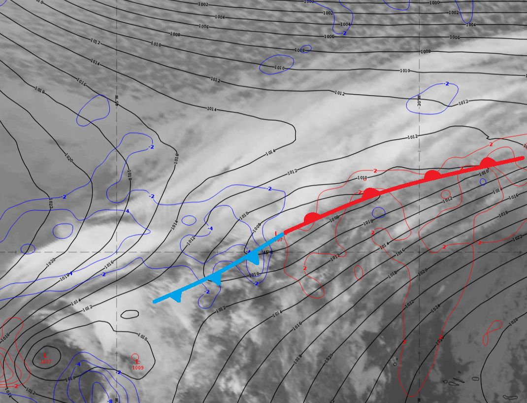
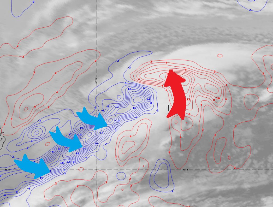
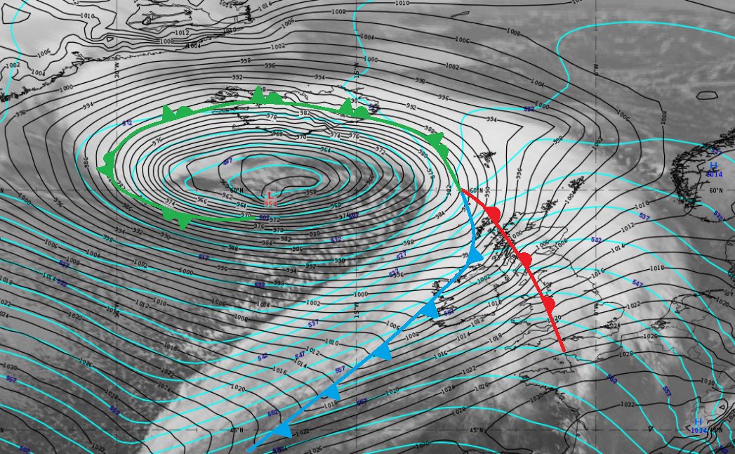
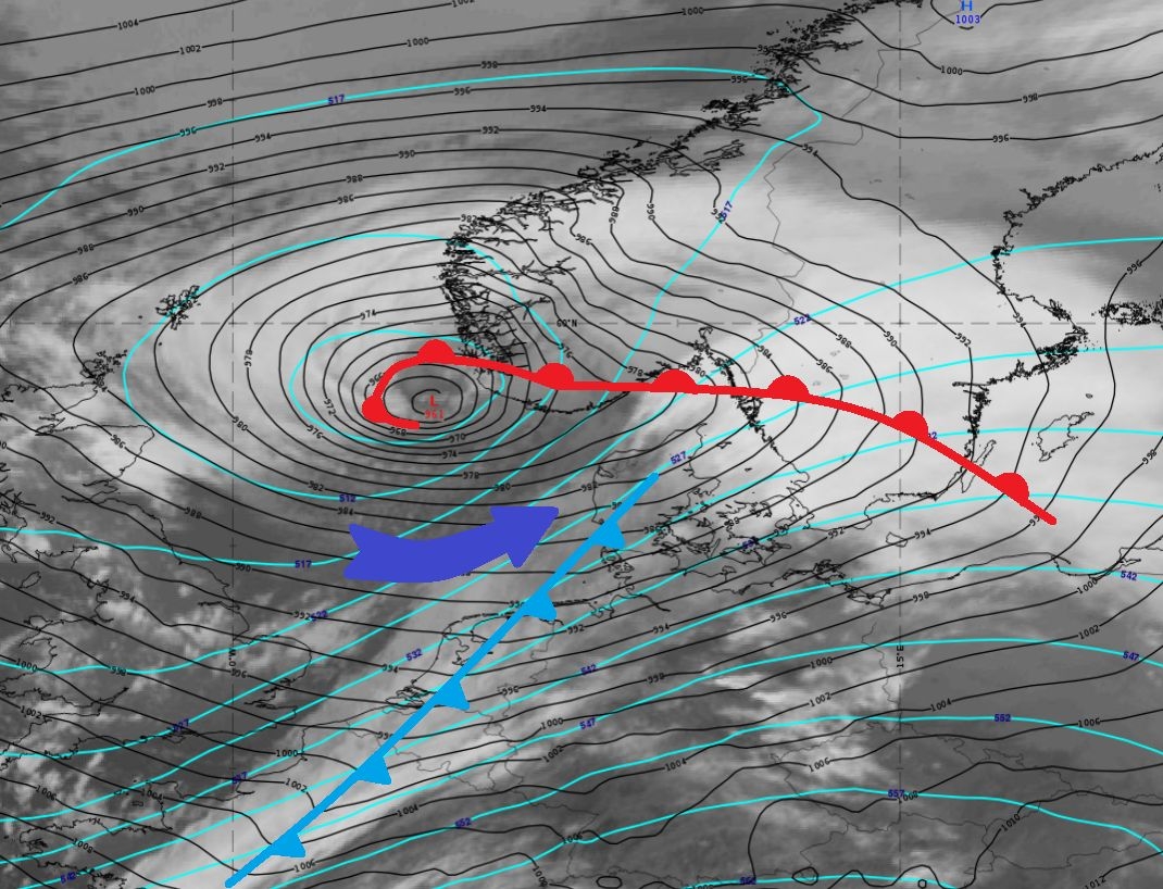
Shapiro-Keyser Cyclone (S-K) During maturity stage, the warm core of the Shapiro-Keyser cyclone becomes secluded from the warm sector. Cold air from behind the cold front protrudes northeastwards (blue arrow), starting from upper levels and protruding towards lower levels. The protruding cold air extends the cold front towards the warm front; the warm and cold front form a right angle, the so-called T-bone pattern characteristic of S-K cyclones. There is no occlusion at this stage of development. |
|
Figure 1a: SEVIRI IR10.8 μm image. Mean sea level pressure (black) and geopotential height at 500 hPa (cyan). The temperature charts at different levels show a tongue of warm air forming the occlusion cloud band. This warm air originates from the warm sector and is advected around the low-pressure center. The cold and warm front are well delimited by the temperature gradient, which is stronger for the cold front. |
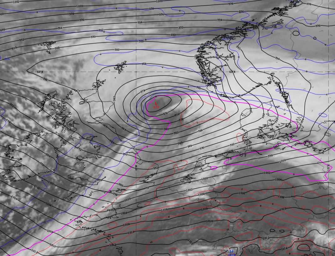
Figure 1b: SEVIRI IR10.8 μm image. Mean sea level pressure (black) and geopotential height at 500 hPa (cyan). The temperature chart at 700 hPa shows the frontal fracture over Denmark; here the temperature gradient of the cold front weakens considerably. The core of the S-K cyclone is filled with warm air, and cold air protruding from behind the cold front in northeastward directions will soon seclude the cyclone's warm core. |
|
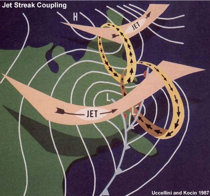
Figure 2a: SEVIRI IR10.8 μm. Blue lines indicate the temperature at 700 hPa. The jet axis still runs along the rear side of the cold front, but the surface pressure minimum is no longer located in the left-exit quadrant of the jet. Another branch of the jet has formed along the leading edge of the warm front. The axes of the two branches are perpendicular to each other (blue lines in Figure 3a). |
Figure 2b: SEVIRI IR10.8 μm. Blue lines indicate the temperature at 700 hPa. The two branches of the jet streak in S-K cyclones form an obtuse angle (> 90°). This is favorable for coupling of the jet streaks, which leads to a more effective triggering of the development of the surface low. The jet axes are almost in line with each other (blue lines in Figure 3b). |
|
Figure 3a: SEVIRI IR10.8 μm image. Mean sea level pressure (black) and isotachs at 500 hPa (yellow). Vertical cross section: A vertical cross section through the occlusion cloud band of the Norwegian cyclone shows the wedge of warm air as a V-shaped pattern in the equivalent potential temperature field. Compared to the warm air from the warm sector that forms the occlusion cloud band, the air within the core of the cyclone is colder. |
Figure 3b: SEVIRI IR10.8 μm image. Mean sea level pressure (black) and isotachs at 300 hPa (yellow). Vertical cross section: The vertical cross section through the warm core of the S-K cyclone shows two distinct frontal zones: a cold front (blue) and another frontal zone delimiting the warm core from the cold air in the north (red). This second frontal zone shows clear warm front characteristics, for which reason Shapiro and Keyser denoted it as a warm front and not as an occlusion. |
|
Figure 4a: SEVIRI IR10.8 μm image with a yellow line indicating the position of the vertical cross section, blue lines indicate the temperature at 700 hPa. |
Figure 4b: SEVIRI IR10.8 μm image with a yellow line indicating the position of the vertical cross section, blue/magenta lines indicate the temperature at 850 hPa. |
|
Figure 5a: Cross section (south-west to north-east) from the ECMWF model. |
Figure 5b: Cross section (north-west to south-east) from the ECMWF model. |

Quiz:
What forms the T-bone structure in the case of a S-K cyclone? Select only one answer!
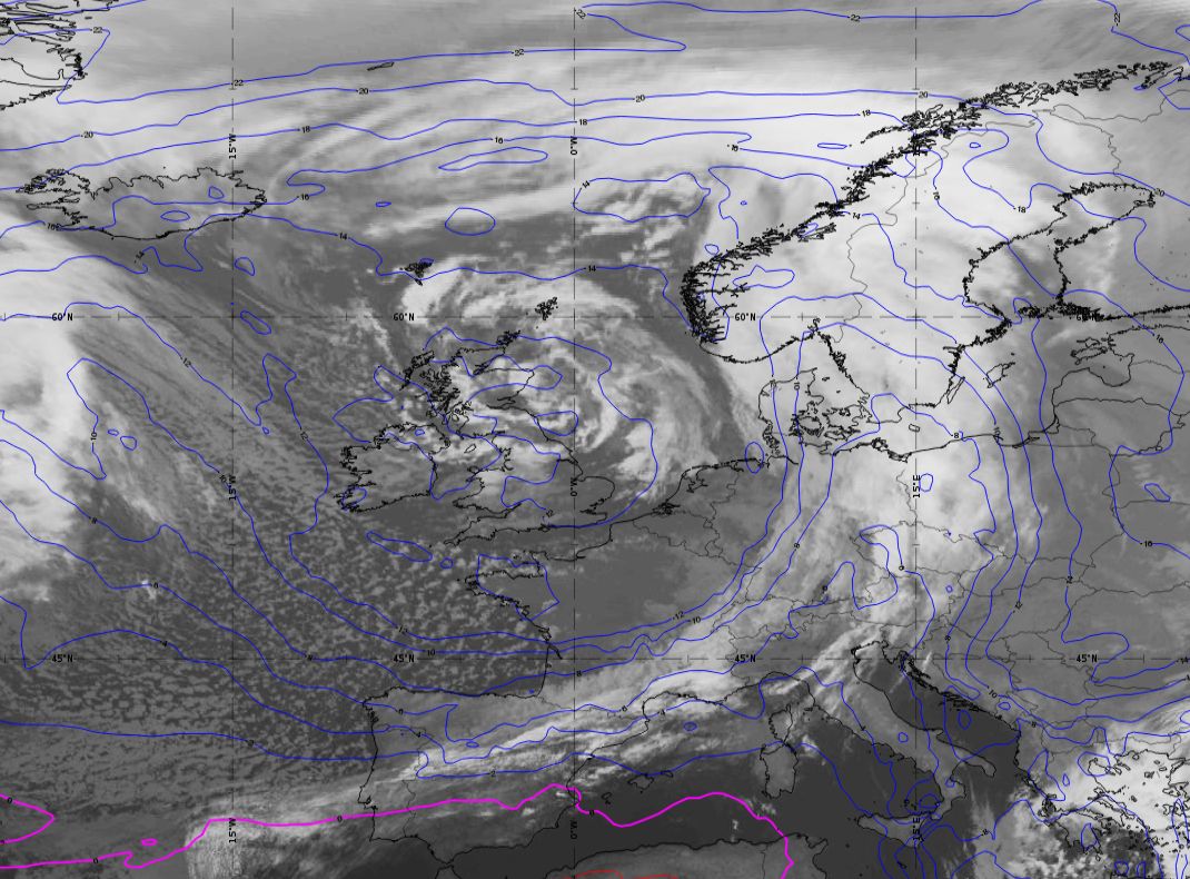
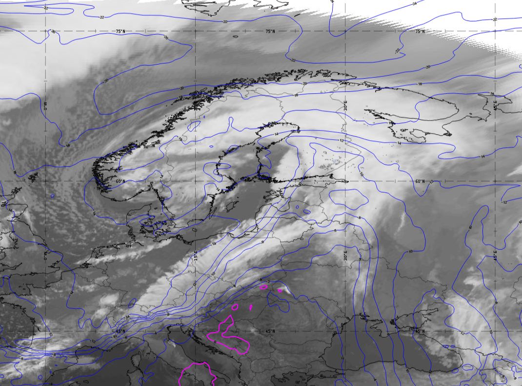
E) Dissipating stage
The dissipating stage is characterized by a temperature adjustment between the polar and tropical air masses. While for the Norwegian cyclone type, the warm air from within the occlusion cloud band mixes with the polar air mass, for Shapiro-Keyser cyclones, the warm core adjusts towards the surrounding cold air. In both cases, the result of the physical processes is a temperature adjustment between polar and tropical air masses.
|
Norwegian Cyclone During the dissipating stage, the surface low begins to fill up and the center pressure increases again. The warm air of the occlusion cloud band mixes with the surrounding cold air and temperature gradients disappear within the polar air mass. The core of the Norwegian cyclone is in the cold air and the temperature difference between polar and tropical air has been reduced. The occlusion cloud band wrapped around the low starts to dissolve. As a result, parts of the cloud band become invisible in IR imagery, as in this example. |
Shapiro-Keyser Cyclone (S-K) During the dissipating stage, protruding cold air from behind the cold front wraps around the warm core of the S-K cyclone. The warm core of the cyclone is located in the polar air mass and the temperature gradient to this surrounding colder air mass decreases. Aging Shapiro-Keyser cyclones show physical processes typical for Norwegian cyclones, like the merging of the warm and the cold front to form an occlusion. This is the case when cold air from behind the cold front wraps around the warm core. Subsequently, the cold front connects to the warm front (closing the cold frontal fracture) and forms an occlusion. |
|
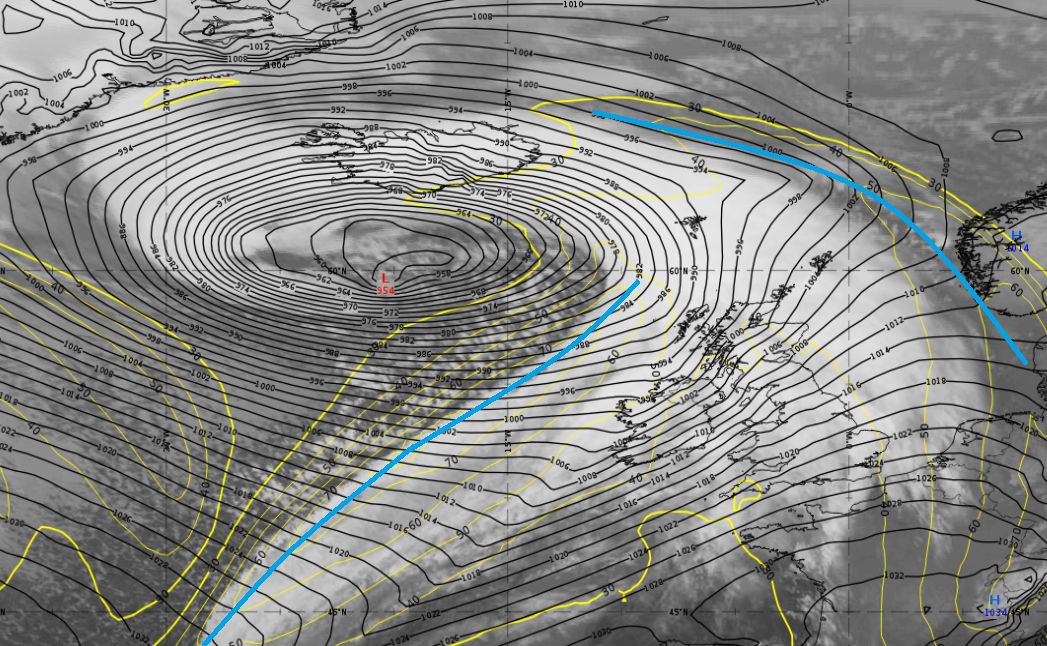
Figure 1a: SEVIRI IR10.8 μm image. Mean sea level pressure (black) and geopotential height at 500 hPa (cyan). The dissolving occlusion cloud band leads to a temperature adjustment between the polar and tropical air masses. |
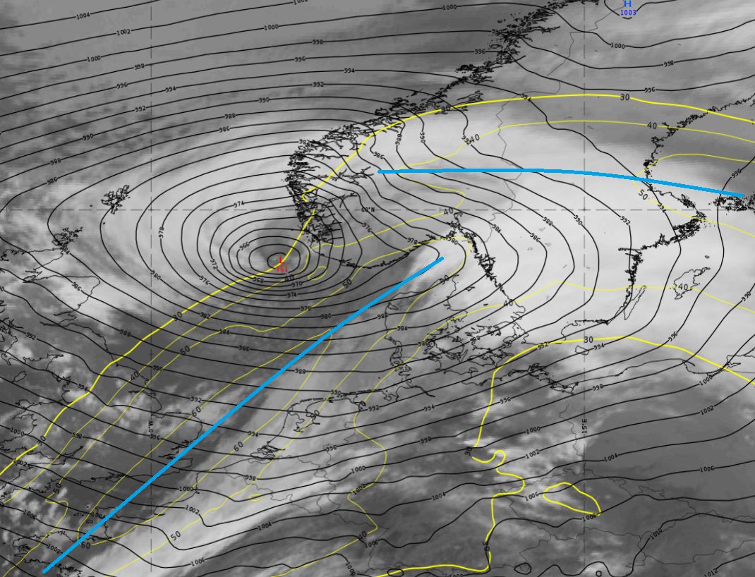
Figure 1b: SEVIRI IR10.8 μm image. Mean sea level pressure (black) and geopotential height at 500 hPa (cyan). The warm core of the Shapiro-Keyser cyclone intermixes with the surrounding cold air at the end of its life cycle. |
|
Figure 2a: SEVIRI IR10.8 μm. Blue/magenta lines indicate the temperature at 700 hPa. The left-exit quadrant of the jet is no longer superimposed on the surface pressure minimum; upper-level divergence ceases to act as a trigger for the surface low. |
Figure 2b: SEVIRI IR10.8 μm. Blue/magenta lines indicate the temperature at 700 hPa. The left-exit quadrant of the jet is no longer superimposed on the surface pressure minimum; upper-level divergence ceases to act as a trigger for the surface low. The two jet streaks are aligned at a more acute angle then before. |
|
Figure 3a: SEVIRI IR10.8 μm image. Mean sea level pressure (black) and isotachs at 300 hPa (yellow). Blue lines indicate the jet axis. Vertical cross section: The vertical cross section through the core of the Norwegian cyclone shows a uniform temperature pattern. Only the northern part of the occlusion cloud band between Iceland and Norway still shows a strong temperature gradient. |
Figure 3b: SEVIRI IR10.8 μm image. Mean sea level pressure (black) and isotachs at 300 hPa (yellow). Blue lines indicate the jet axis. Vertical cross section: A vertical cross section through the region where the warm and cold fronts merge shows the typical pattern of an occlusion with warm front character; the cold front does not reach the ground and the surface front is a warm front. In this example, the warm front exhibits a double structure. |
|
Figure 4a: SEVIRI IR10.8 μm image with a yellow line indicating the position of the vertical cross section, mean sea level pressure (black) and geopotential height at 500 hPa (cyan). |
Figure 4b: SEVIRI IR10.8 μm image with a yellow line indicating the position of the vertical cross section, mean sea level pressure (black) and geopotential height at 500 hPa (cyan). |
|
Figure 5a: Cross section (north to south) from the ECMWF model. |
Figure 5b: Cross section (south-west to north-east) from the ECMWF model. Another vertical cross section, through the boundary that wraps around the core of the S-K cyclone, shows the typical pattern of a slow-moving front: a weak inclination of the equivalent potential temperature and weak warm air advection. |
|
Figure 6b: SEVIRI IR10.8 μm image with a yellow line indicating the position of the vertical cross section, mean sea level pressure (black) and geopotential height at 500 hPa (cyan).
Figure 7b: Cross section (southeast to north-west) from the ECMWF model. |
Quiz:
What is the driving force that causes the dissipation of both cyclone types? Select only one answer!
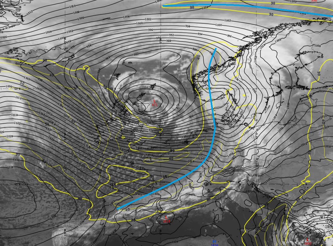
Quiz:
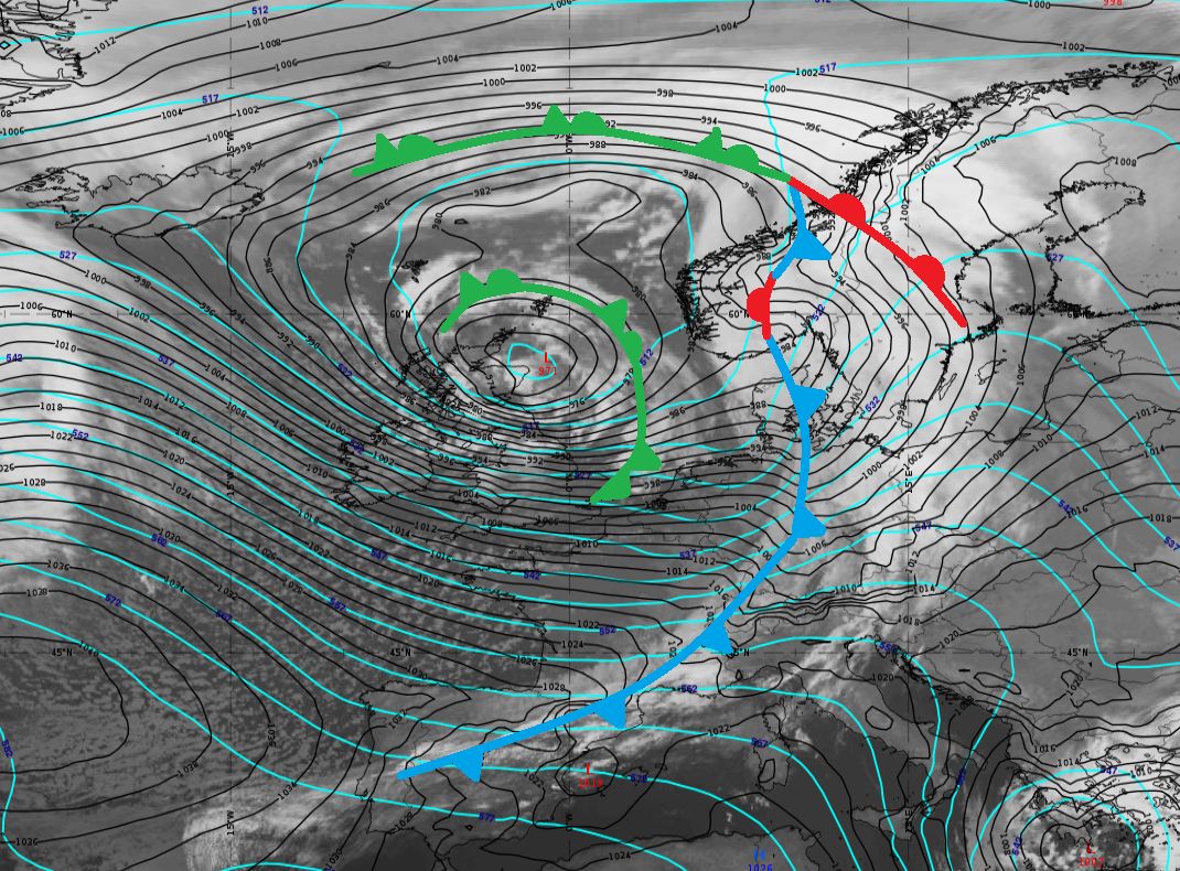
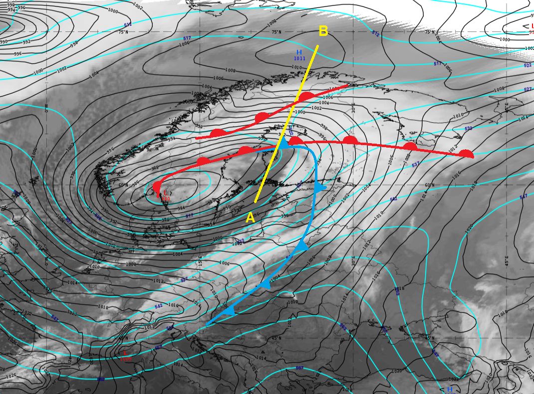
Make a frontal analysis of this cyclone by using the NWP charts provided.
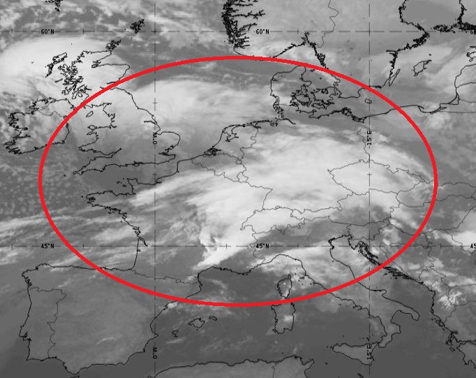
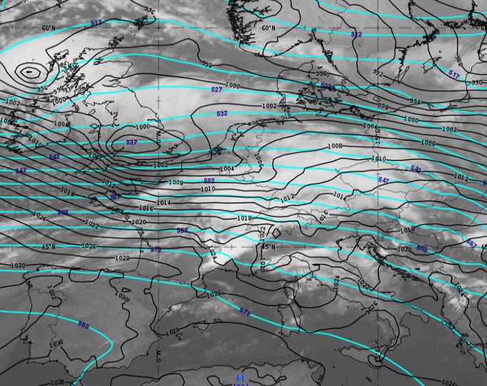
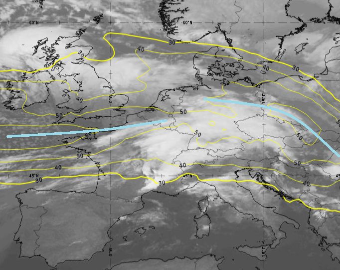
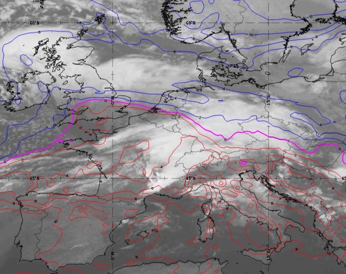
Figure 1: SEVIRI IR10.8 μm image from 10 March 2019; 06:00 UTC.
Top left: the red circle delimits the cyclone. Top right: mean sea level pressure (black) and geopotential height at 500 hPa.
Bottom left: isotachs at 300 hPa (yellow) and jet axis (blue). Bottom right: temperature at 850 hPa (blue/magenta).
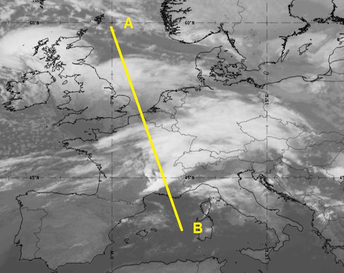
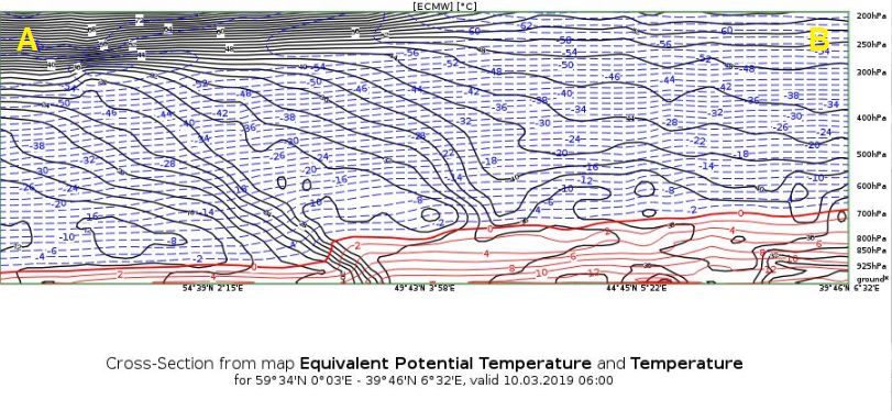
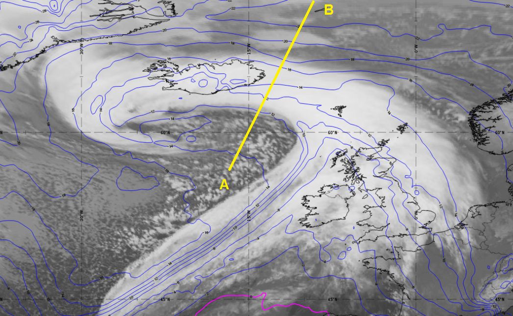
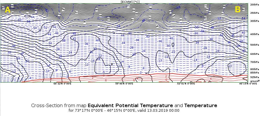
Figure 2: SEVIRI IR10.8 μm image from 10 March 2019, 06:00 UTC; the yellow line (left) marks the position of the vertical cross section (right).
When ready for the solution, click Ready!