The sting jet question
High 10 m wind speeds (20-22 m/s) could already be analysed in the warm sector of the cyclone, prior to its rapid deepening (Fig. 4.1).
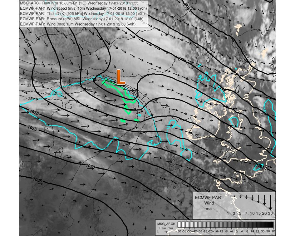
Figure 4.1: METEOSAT IR10.8 image (background), ECMWF 10 m wind speed (coloured lines at 15 and 20 m/s), mean sea level pressure (thick lines, hPa), potential temperature (dashed lines), 10 m wind (arrows). Note the high 10 m wind speed in the warm sector of the cyclone, close to its centre.
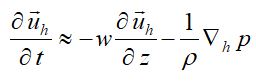
The wind speed at 950 hPa (400-500m ASL) reached 30-35 m/s over a large territory. It is probable that this high wind speed was largely due to a high pressure gradient and pressure gradient force (PGF). Besides PGF, vertical advection of momentum causes increases in horizontal wind speed (Slater et al., 2015):
 , (Eq.2)
where the left-hand side of Eq. 2 represents the local tendency of the horizontal wind vector, the first term on the right-hand side the vertical advection of momentum and the second term on the right-hand side the pressure gradient force effects. It can be shown that in the momentum tendency equation only these two terms can contribute to acceleration of the wind (other terms, like horizontal advection of momentum or the Coriolis force term either do not cause acceleration or decelerate the wind and are not shown). The magnitude of the momentum tendency created by the vertical advection term depends both on vertical velocity and wind shear (the latter was very high in the low and mid-troposphere in our case). These two effects are not necessarily independent, because increases in downward vertical motion cause the pressure and pressure gradient to rise; in our case this was also demonstrated by maxima in the pressure tendency (6 hPa in 3 h) at the western and southwestern side of the low.
During the rapid deepening phase, significant mid- and low-level downward motion occurred in the neighbourhood of the cold conveyor belt (over the North Sea), which was suggested by several models (ECMWF, ALADIN). The speed was typically from 1 to 2 Pa/s (roughly between -0.1 and -0.2 m/s), which is slower than downdrafts typically produced by deep convection or symmetric instability, but it could have been sufficient to transport the high upper-air momentum toward the top of the planetary boundary layer (PBL). At the same time, a continuous increase in 10 m wind speed could be observed downstream of the above-mentioned vertical velocity maxima (Fig. 4.2).
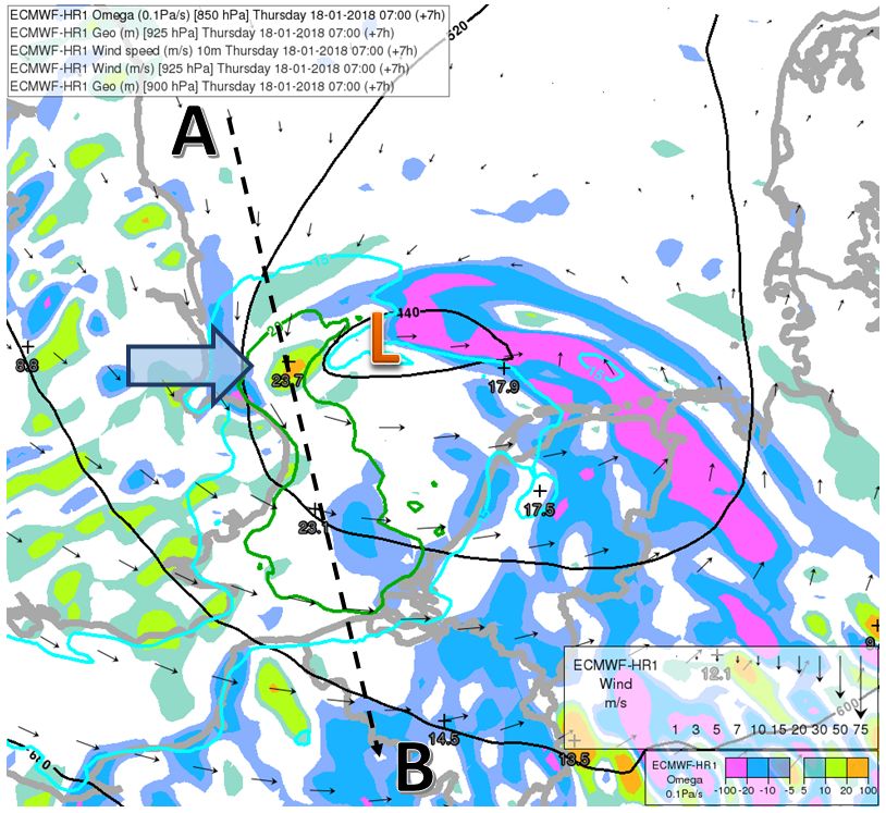
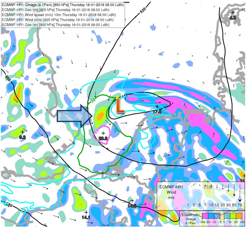
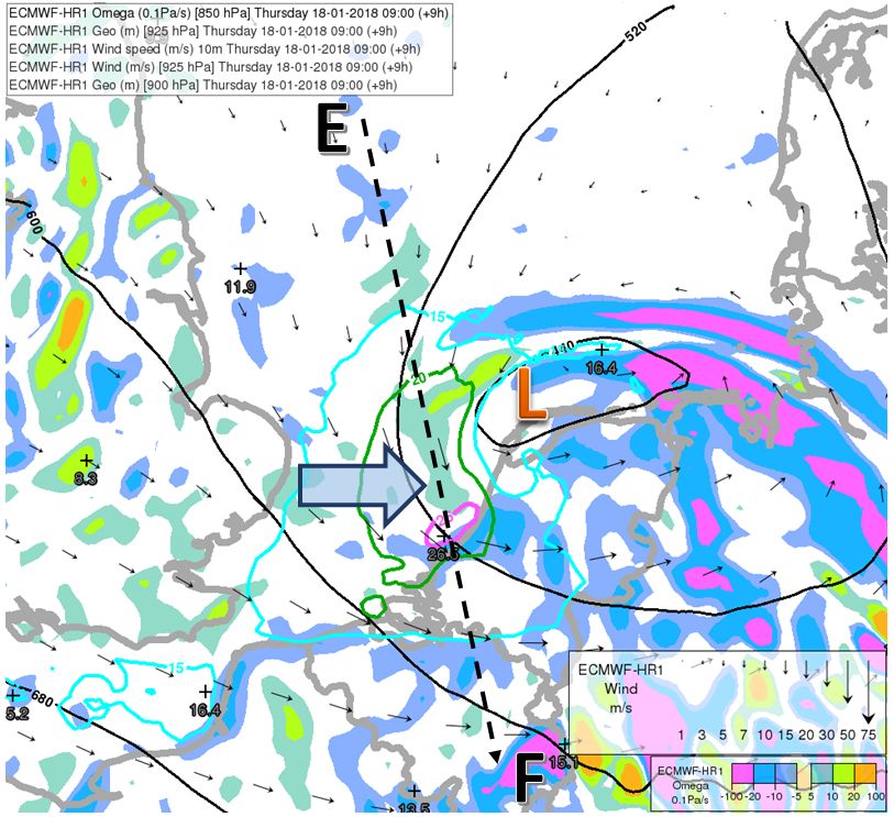
Figure 4.2: a) Upper left: ECMWF 7 h forecast of vertical motion (colour shades, 0.1 Pa/s), 925 hPa geopotential (black lines, gpm), 10 m wind speed (coloured lines at 15, 20, 25 m/s) and 925 hPa wind (arrows), valid for 18 January 2018 07 UTC. The AB line shows the position of the cross-section in Fig. 4.3a. The large arrow points toward the position of stronger downward motion (2.37 Pa/s) at the rear of the cyclone.
b) Upper right: as in a) but for 08 UTC. Strengthening of the 10 m wind is visible by the appearance of wind speeds exceeding 25 m/s (magenta line) downstream of the downward motion.
c) Bottom: as in the previous two figures but for 09 UTC. The 25 m/s wind speed reached the coast of the Netherlands, but the downward motion became weaker. The EF line shows the position of the cross-section in Fig. 4.3b.
From Eq. 2 it can be estimated that a downdraft of this strength could result in further increases in wind speed by 2-4 m/s during a one-hour period. The extension of the high wind speed from mid-levels to close to the surface can be seen on the vertical cross-sections (Fig. 4.3) as well.
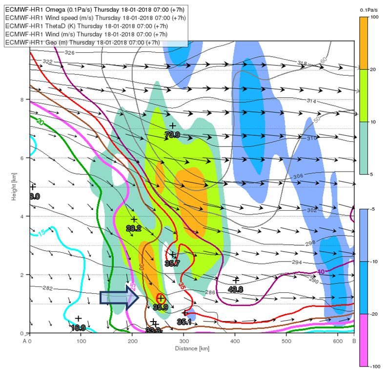
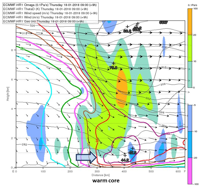
Figure 4.3: a) Left: AB vertical cross-section (its position is depicted in Fig. 4.2a) in the ECMWF forecast of vertical motion (colour shades, 0.1 Pa/s), potential temperature (thin solid lines, K), wind speed (coloured solid lines, m/s), wind (arrows), valid for 18 January 2018 07 UTC. The large arrow points toward a region of slanted isentropes and sinking motion at low levels. A wind maximum (exceeding 35 m/s) developed in this region.
b) Right: as in a) but for the EF section (its position is depicted in Fig. 4.2c) and 2 h later. The low-level wind speed became even stronger (40 m/s below 1 km height). Note the convex curvature of the isentropes in this region, which appeared as a warm core on the horizontal potential temperature sections.
The cross-sections show that there was probably a strong link between this extension and slanted downward motion between 1 and 4 km height. The sinking mid-level air was also relatively dry (relative humidity well below 50%). It could be expected that locally stronger downward motion would cause dissipation of low-level clouds, as seen on 18 January, at around 10 UTC, on the satellite imagery (Fig. 4.4).
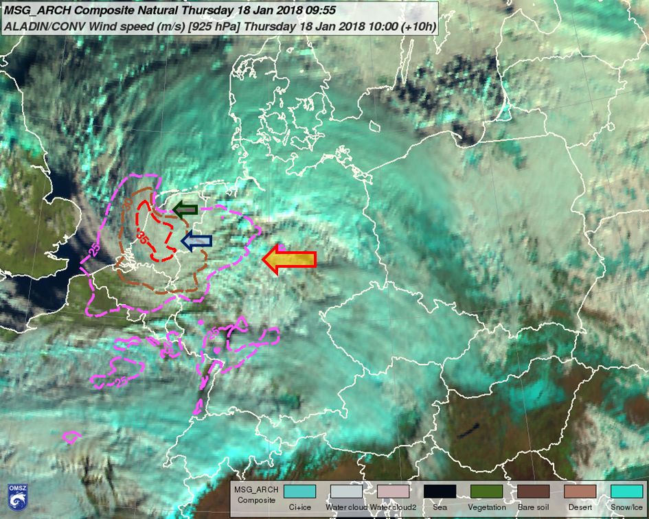
Figure 4.4: METEOSAT Natural Colour RGB image (background) for 18 January 09:55 UTC and ALADIN-HU model (run at OMSZ) forecast of 925 hPa wind speed (lines, m/s), valid for 18 January 10 UTC. The top of the cloud bands (marked by the large arrow) include ice/snow particles (and probably also supercooled water drops according to the Day Microphysics RGB images). These clouds were precipitating (according to OPERA radar imagery, which is not shown) and were situated at the cyclone's cold front, or just ahead of it. The NWC SAF cloud top height suggested a 3 km height or somewhat above (see also the caption of Fig. 5.2). One could find shallow convective water clouds in the areas of strongest gusts over the Netherlands (marked by the smaller arrow), whose tops were nearly at 2 km height. The small green arrow points toward the end of the cloud-head, where a hole in the cloudiness started to form. Cloud dissipation was also visible over the North Sea, northwest of the coast of the Netherlands.
The strongest wind gusts in rapidly developing cyclones are often attributed to the sting jet phenomenon. The sting jet is caused by downslope motion at the end of the cyclone's occlusion and causes very high winds in a narrow (few tens of kilometres wide) swath (Fig. 4.5).
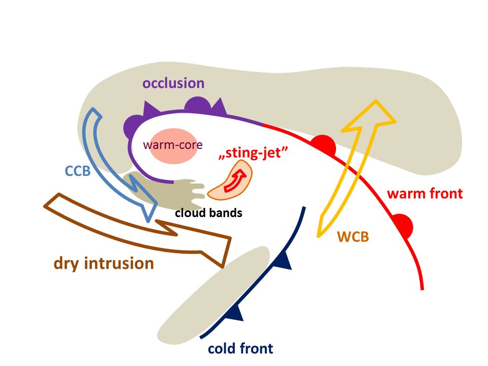
Figure 4.5: Schematic of a cyclone with possible sting jet development (adapted from Clark et al., 2005). Some features (warm core in the potential temperature field, dry air intrusion, parallel cloud bands) also occurred in the Friederike cyclone. However, the presence of a sting jet corresponding to the original conceptual models is only hypothetical.
Such severe gusts were, for example, produced by the 16 October 1987 cyclone, when the peak gust reached 190 km/h. For some time, the existence of the sting jet was explained by the presence of conditional symmetric instability (CSI) in its environment. This kind of instability can produce strong (several m/s) downslope motion. It is also often observed, in deep intense cyclones, that the end of the occlusion is characterized by parallel cloud bands, which is a typical feature appearing when symmetric instability is present (Fig. 4.6). However, some scientists currently admit that symmetric instability is not a necessary condition for development of a sting jet or a sting-jet-like flow. It is also important to note that strong gusts in deep cyclones can be produced by several kinds of process (deep convection, turbulence, mountain wave effects, etc.).
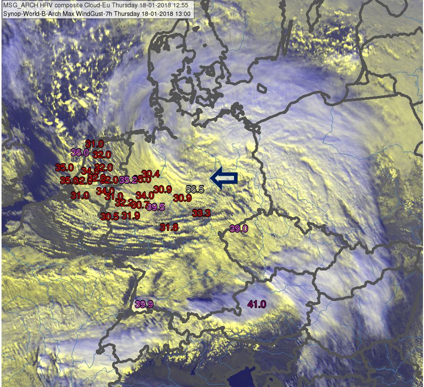
Figure 4.6: METEOSAT HRV Cloud RGB (background) on 18 January, at 12:55 UTC, and maximum wind gusts (depicted in numbers, only those exceeding 30 m/s) from meteorological station observations reported between 06 and 13 UTC. The arrow points toward the parallel cloud bands south of the cyclone's centre. Most of the strong gusts occurred south or southwest of the cloud band, unlike in the conceptual model in Fig. 4.5. The strongest gust (56.5 m/s) shown here appeared at the station at Brocken, which is 1142 m high.
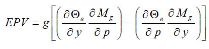
The equivalent potential vorticity (EPV) is sometimes used for visualization of the conditional symmetric instability. Its definition yields:
![]() , (Eq.3)
, (Eq.3)
where ηg is the geostrophic absolute vorticity vector and θe is equivalent potential temperature.
For a two-dimensional flow this equation has the following form:
 , (Eq.4)
where Mg is the absolute geostrophic momentum derived from the geostrophic wind component ug, Coriolis parameter f and the y-coordinate of a two-dimensional cross-section pointing toward a warmer airmass (Mg = ug - fy). Eq. 4 shows that negative EPV can be found if θe lines are steeper than Mg lines (and there is neither convection nor inertial instability). Areas of negative EPV could be found in the occlusion belt of the Friederike cyclone at mid-levels (Fig. 4.7a). The east-west cross section of θe and Mg enabled the identification of areas with CSI (Fig. 4.7b). These could be found at 3-4 km height, above the strongest diagnosed vertical motion highlighted in Figs. 4.2 and 4.3. At low levels, the EPV was still negative but the Mg lines were almost vertical, which makes the identification of CSI ambiguous.
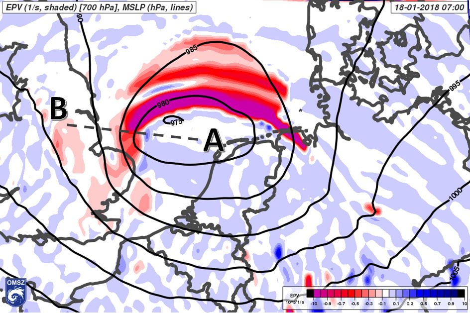
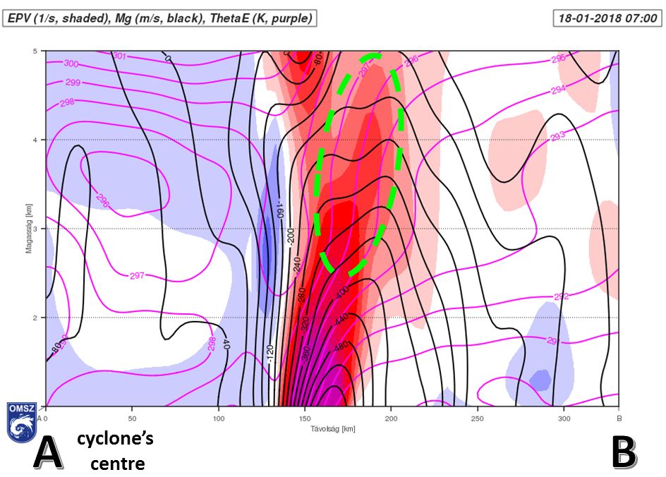
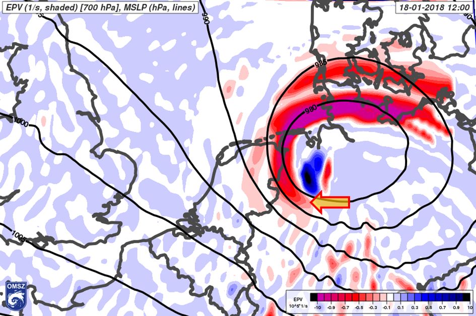
Figure 4.7: a) Top left: ECMWF 7 h forecast of 700 hPa equivalent potential vorticity (EPV, shades, 10-5 1/s) and mean sea level pressure (lines, hPa), valid for 18 January 2018 07 UTC. The A-B line shows the position of the east-west cross-section in Fig. 4.7b.
b) Top right: East-west vertical cross-section through the fields of EPV (shades), absolute momentum (Mg, black lines) and equivalent potential temperature (magenta line). The thick dashed green line emphasizes an area with conditional symmetric instability. In this region, the Mg lines were less vertical and the θe lines were steeper than the Mg contours. The 0-1 km part is omitted due to artefacts in the EPV field near the ground.
c) as in a), but valid for 18 January 2018 12 UTC. The arrow points toward the region with conditional symmetric instability at mid-levels.
In later hours, the negative EPV area moved with the cyclone but it remained rather on its rear and southern flank. The width of the negative EPV belt was approximately 50 km. This indicates that, even if CSI could have played a role in the generation of downward vertical motion and transport of momentum toward low tropospheric levels, the swath of strong gusts actually observed was simply too wide to be attributed to this phenomenon only.
According to the original sting jet conceptual model we should find the strongest gusts downstream of the parallel cloud bands visible on Fig. 4.6. Based on the EPV diagnostics and cross-sections, the sting-jet-related up- and downward motion would develop somewhere at the end of the cold conveyor belt but rather at mid-levels. The available observations also do not show that the strongest gusts occur close to the cyclone's centre, as suggested by some sting jet conceptual models. The observed gusts can be mostly explained by the existence of strong low-level (e.g., in the lowest 100 hPa) wind advected from the west and intense turbulent transport of momentum toward the surface (more details in the next section) even without the presence of CSI. However, the simultaneous impact of symmetric instability flow on surface wind acceleration is not excluded for certain areas. For example, there were isolated very strong gusts over eastern Germany, close to the above-mentioned parallel band of clouds visible in the HRV Cloud RGB satellite imagery (although appearing rather over mountains). To prove the existence of CSI with available observations or even with numerical simulations is rather difficult. Even if this instability was present, it is uncertain whether it was also released and whether the resulting flow reached the surface or the PBL top. It is also often observed that symmetric instability exists only for a relatively short period, before transforming into convective (conditional) instability.