Early development
Although the rapid deepening of the cyclone started over the British Isles, its origin could be traced far upstream. On 15 January 2018, a deep trough of low pressure was situated east of the Florida coast (Fig. 2.1).
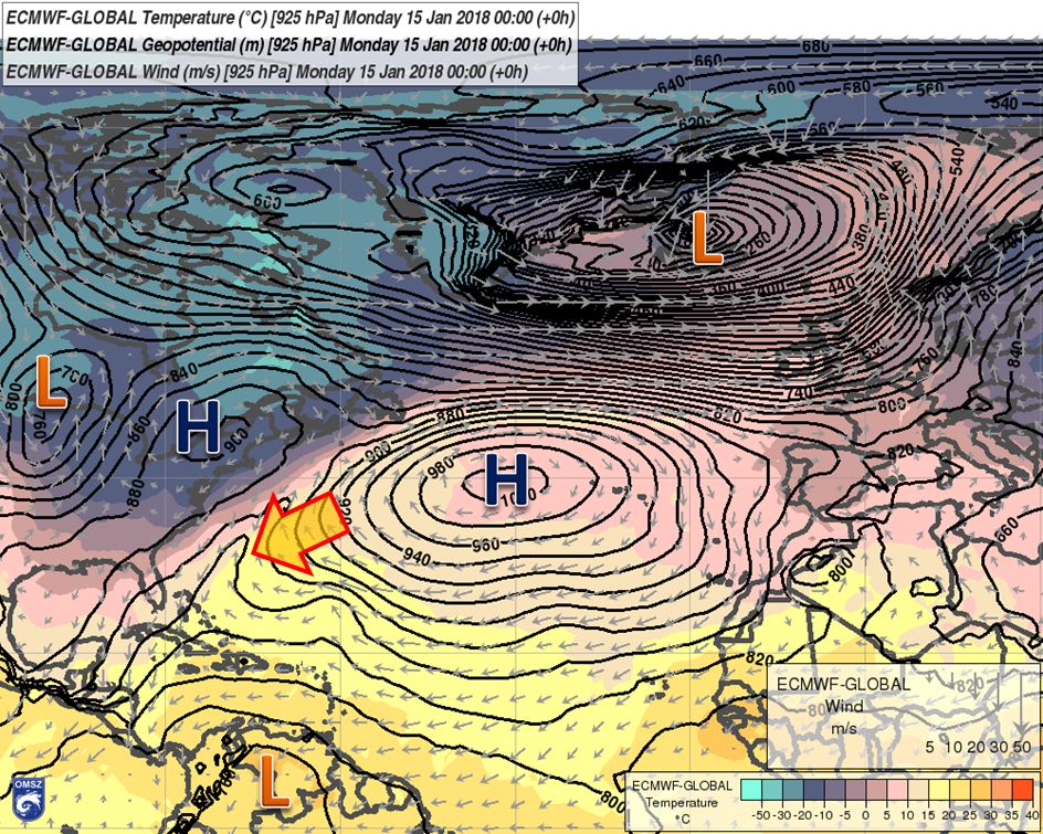
Figure 2.1: ECMWF 925 hPa temperature (colour shading), geopotential (lines) and wind (arrows) analysis valid for 15 January 2018 00:00 UTC. The large arrow points toward the origin of the Friederike cyclone, a trough east of the Florida peninsula. The cyclone developed from this trough and moved north-eastward.
There was a very cold airmass over the eastern part of the United States (the ECMWF analysis indicated large areas below -10 °C at 925 hPa). On the other hand, much warmer air (above 15 °C) started to flow northward on the southwestern flank of a large anticyclone over subtropical regions of the Atlantic. A well-defined baroclinic zone thereby came into existence, in which the trough transformed into a cyclone (Fig. 2.2) moving in the north-north-eastward direction.
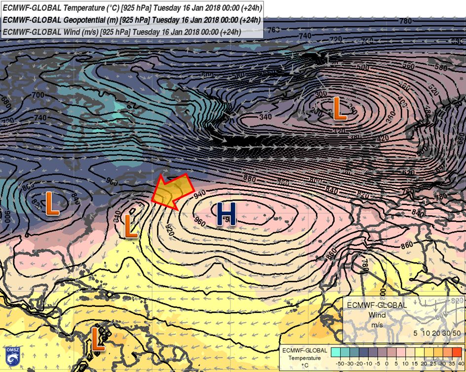
Figure 2.2: As in Fig. 2.1, but for 16 January 2018 00 UTC. Note the development of a low in the 925 hPa geopotential field at the eastern coast of the USA (indicated by the arrow).
On 16 January 2018, the cyclone was close to the entrance region of a very strong upper-air jet, which stretched from the Labrador Peninsula up to the British Isles (Fig. 2.3a). This strong westerly upper-air flow had an important role in the later propagation and development of the cyclone (Fig. 2.3b).
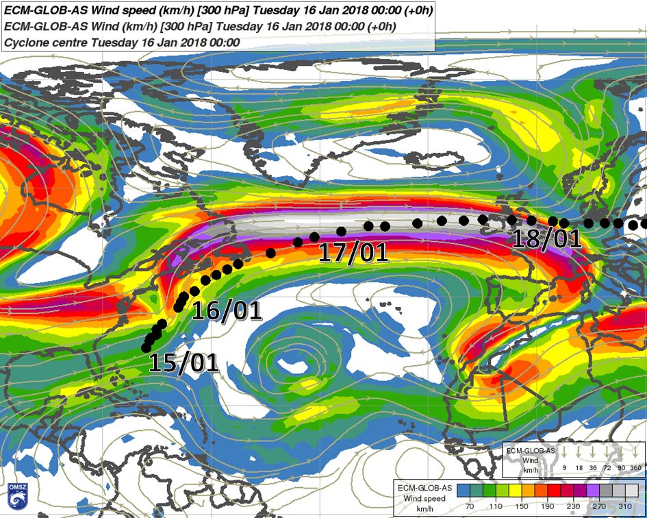
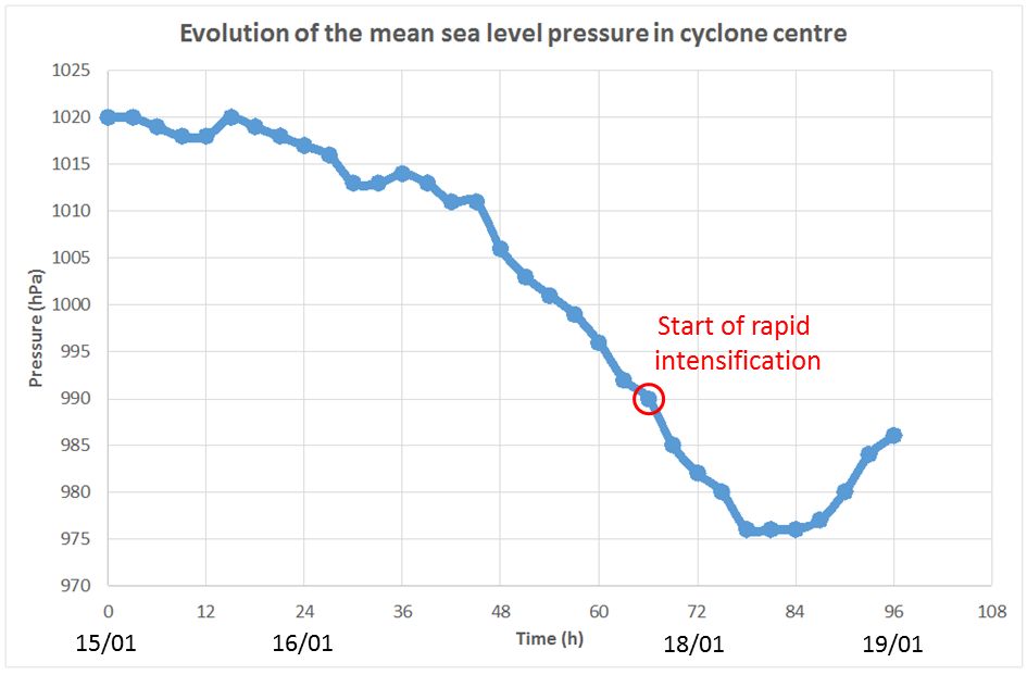
Figure 2.3:
a) Left: ECMWF 300 hPa windspeed (colour shading) and streamlines from the 16 January 2018 00 UTC analysis. The polar jet stream over the Atlantic Ocean is clearly visible. The dots show the position of the cyclone centre (minimum in mean sea level pressure) from 15 January 2018 00 UTC until 19 January 2018 00 UTC at 3 h intervals.
b) Right: Development of the mean sea level pressure in the cyclone centre during the above-mentioned period. We denote the start of rapid intensification (around 17 January 2018 18 UTC), which refers to a change in the cyclone's structure and an amplification of vertical motion (discussed later in the text).
On 17 January 2018, the cyclone started to propagate eastward, on the anticyclonic side of the jet. However, it was still rather shallow, and it became part of a larger cyclonic circulation over the North Atlantic, which had already developed several days earlier. During this stage, it was still questionable from a forecasting point of view whether it would reach the British Isles as an independent surface cyclone or only as a trough of lower pressure (see the extended discussion in Section VI). One problem is that there are fewer surface pressure observations or soundings over the ocean than over land. Therefore, during this phase, it was necessary to rely to a great extent on model output. One possibility for monitoring the evolution of a cyclone is to compare NWP charts of diagnostic parameters (e.g. Q vector or PV fields) with satellite imagery. According to quasi-geostrophic theory (see Eq. 1), Q-vector convergence implies the presence of mid-level ascending motion, which is important for the maintenance of a cyclone:
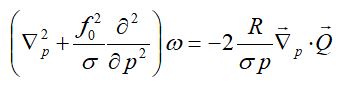 , (Eq.1)
where f0 is the Coriolis parameter, σ is the static stability parameter, ω is the vertical velocity in pressure coordinates and is the Q⃗ vector.
As an example of this, for the Friederike case, the Q-vector diagnostics showed convergence in the cyclone's centre and in the cloud head, where cold cloud-tops could be seen on the satellite image (Fig. 2.4). On the other hand, Q-vector divergence occurred on the rear side of the cyclone, where the cloudiness dissipated.
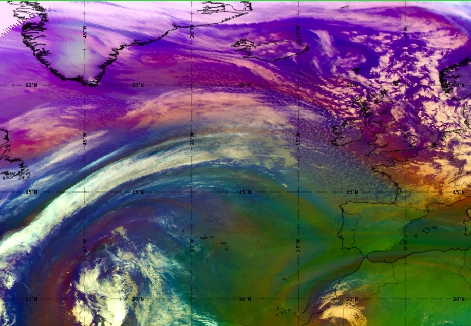
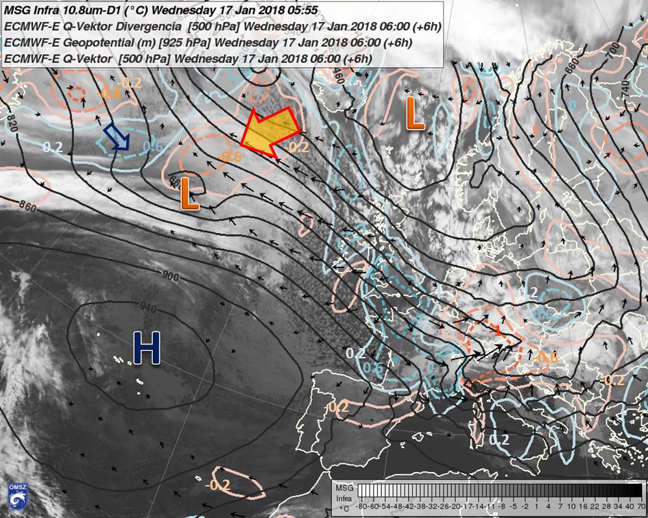
Figure 2.4:
a) Left: Airmass RGB taken on 17 January 2018 at 06:00 UTC.
b) Right: METEOSAT IR10.8 image (background), ECMWF Q-vector (vector field) and Q-vector divergence (coloured lines) forecast valid for 17 January 2018 06:00 UTC. Based on quasi-geostrophic theory, Q-vector convergence (reddish lines, 10-12 m3s/kg) indicates frontogenesis and generation of ascending motion, while divergence (bluish lines, 10-12 m3s/kg) means frontolysis and downward motion. Although the cyclone became part of a pre-existing large cyclonic area, situated north of the polar jet stream (not shown here), diagnostic parameters indicated significant generation of upward motion in its head (emphasized by the large arrow). Downward, frontolytic motion existed in its rear part and behind the cold front (smaller arrow), where the cloudiness dissipated.
Concerning the structure, some features could be recognized, which frequently occur in extratropical cyclones. One was a band of moist air elongated in the southwest-northeast direction, which could be seen on both water vapour (WV) satellite images and on equivalent potential temperature (θe) charts (Fig. 2.5).
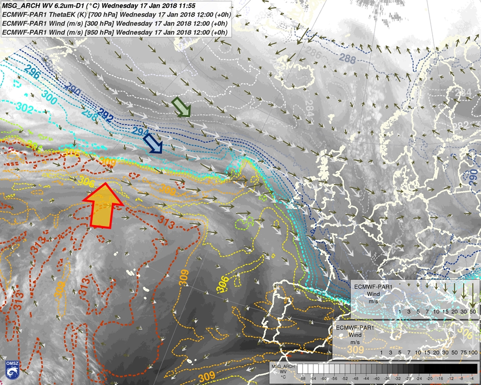
Figure 2.5: METEOSAT WV6.2 image (background), ECMWF 700 hPa equivalent potential temperature ThetaE (coloured lines), 950 and 300 hPa wind (green and white arrows, respectively); forecast valid for 17 January 2018 12:00 UTC. The large arrow points toward the cloudiness of an "atmospheric river" marked by high ThetaE values. Behind the cyclone's cold front, there is a dark stripe in the WV imagery, indicating a slot of dry air at upper levels. The smaller blue arrow points toward this region. Another small (green) arrow points toward the dry air region behind the jet streak, which was of stratospheric origin.
Although it seems straightforward to associate this band with the Warm Conveyor Belt (WCB), a deeper analysis is necessary. Firstly, the position of the moist band and the θe pattern did not completely overlap, because the WCB is typically well defined at mid-levels (3-5 km), while on the WV images we see the upper tropospheric moisture, which was transported at higher levels (around 7 km, see Fig. 2.6a). Secondly, if we overlay the WV images with storm-relative wind on the 300 K Theta surface (Fig. 2.6b), we can see that, contrary to what would be expected in a WCB, there was hardly any north-eastward wind component along the cloud band toward the cyclone's centre. Such paths of high θe or total column water vapour are sometimes called "atmospheric rivers", but it has been shown (Dacre et al., 2015 BAMS) that the high water vapour amounts can also be produced locally, within the frontal system (e.g. due to water vapour convergence ahead of the cold front) and a footprint of this is left as the cyclone travels poleward. Although trajectory calculations (e.g. from the Hysplit model, not shown) indicate that the atmospheric parcels in the "river" travelled several thousands of kilometres from the southwest, their displacement was probably influenced by the evolution and propagation of the whole cyclone and its fronts.
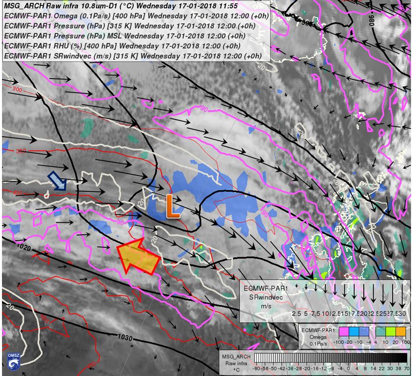

Figure 2.6:
a) Left: METEOSAT IR10.8 image (background), ECMWF 400 hPa vertical motion (Omega, colour shades, Pa/s), 400 hPa relative humidity (light brown line for 20%, magenta line for 90%), mean sea level pressure (thick black lines, hPa), pressure on the 315 K isentrope (red lines, hPa), surface cyclone-relative (storm-relative) wind on the 315 K isentrope (arrows, m/s), valid for 17 January 2018 12 UTC. The large arrow points toward the cloudy region in the cyclone's warm sector, the small arrow toward a dry slot.
b) Right: Similar to a) but for the 300 K isentrope. The vertical velocities represent a 3-level mean (500, 600, 700 hPa). The METEOSAT WV6.2 image is in the background. The large arrow emphasizes the region with ascending motion (storm-relative wind crossing the pressure lines and pointing toward upper levels). The small arrow shows the (initially weak) descending motion on the rear side of the cyclone.
We can also see that there were at least two parallel bands of moisture, which corresponded to two parallel θe gradient zones. A slot of dry air occurred between them, developing behind the cyclone's cold front and entering the frontal system south of the cyclone centre. Such dry slots, cutting off the cloudiness of the cyclone head from its frontal cloud band, can be found in cases with explosive cyclogenesis (Bader et al., 1995). Identification of the WCB using satellite imagery is difficult, because significant southerly storm-relative winds (i.e., relative to the displacement of the cyclone's centre) can only be seen at low levels (e.g., around 925 hPa) and close to the cyclone's centre (Fig. 2.7). The air rose steeply as it approached the warm-frontal boundary; this can also be seen on meridional vertical cross-sections through the fields of relative humidity, potential vorticity, vertical velocity and storm-relative wind components (Fig. 2.8). The very low relative humidity in the dry slot is also clearly visible on the cross-sections. On the potential vorticity (PV) cross-section it can be seen that the frontal zone tilted toward the lower tropopause region to the north of the cyclone.
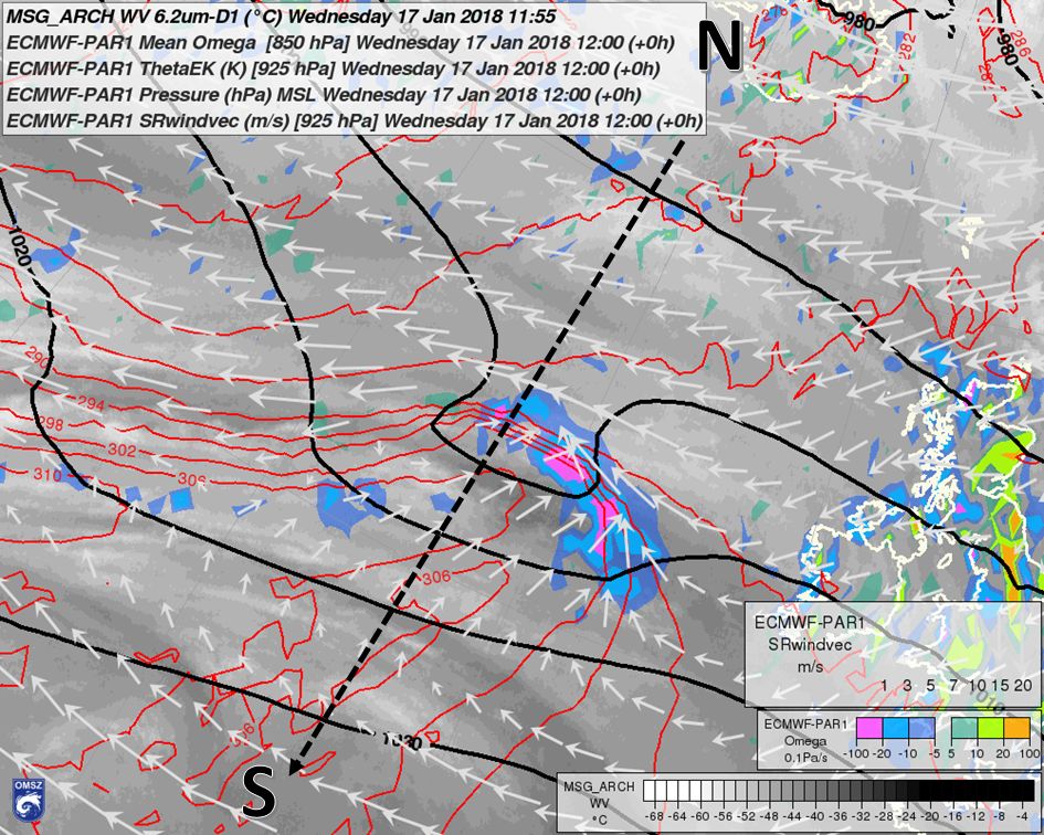
Figure 2.7: METEOSAT WV6.2 image (background), ECMWF mean vertical motion (Omega on 800, 850 and 900 hPa levels, colour shades, Pa/s), 925 hPa equivalent potential temperature ThetaE (coloured lines, K), mean sea level pressure (thick black lines, hPa), surface cyclone-relative wind at 925 hPa (arrows, m/s), valid for 17 January 2018 12 UTC (analysis). The N-S line shows the direction of the North-South cross-section on Fig. 2.8.
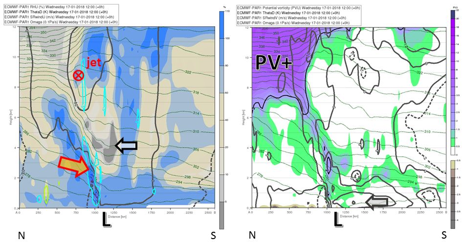
Figure 2.8:
a) Left: North-South cross-section of ECMWF relative humidity (shading, %), potential temperature (contours every 4 K), zonal component of storm-relative wind (only the -20, 0 and 40 m/s isotachs are shown, positive values represent flow into the page, i.e., eastward) and vertical motion (blue and green thick lines, Pa/s, the turquoise -5 Pa/s line represents ascending motion), valid for 17 January 2018 12 UTC (analysis). The large arrow points toward the steep isentropes with strong vertical motion. The smaller arrow shows the position of the mid-level dry slot.
b) Right: The same section but for potential vorticity (PVU, shaded, 2 PVU line emphasized) and meridional component of storm-relative wind (the -2, 0, 5, 10 and 15 m/s isotachs are shown, negative values are dashed). The arrow shows the maximum of the meridional wind component pointing northward (and toward the cyclone centre).
Considering the structure of the frontal system, at this stage it was rather similar to the Norwegian conceptual model, because the temperature gradients were well defined along its cold-frontal part (in potential temperature as well as in equivalent potential temperature). There was an upper-air divergence and frontogenesis close to the cyclone's centre (Fig. 2.9). On 17 January at 12 UTC, the jet streak was still about 300 km north of the centre of the low. It is noteworthy that, on the theta-chart, there was already a significant storm-relative wind component crossing the 300-K-level pressure lines at the rear of the cyclone (refer again to Fig. 2.6). This implies descending motion along the theta-surface toward the cyclone's warm sector, though the resulting downward vertical velocities were not yet very high.
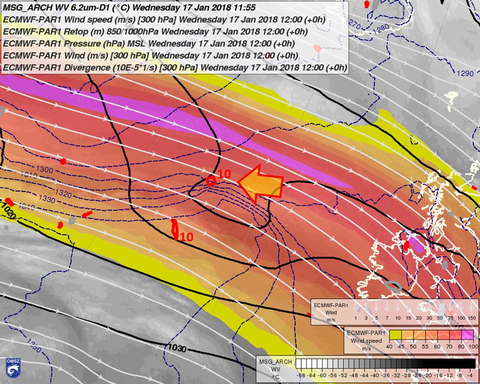
Figure 2.9: METEOSAT WV6.2 image (background), ECMWF 300 hPa wind speed (colour shades, exceeding 40 m/s), streamlines (white lines), divergence (red and grey lines at -10 and 10 x10-5 1/s), 850/1000 hPa relative topography (dashed lines, m), mean sea level pressure (thick lines, hPa), valid for 17 January 2018 12 UTC (analysis). The arrow points toward an area of weak upper-air divergence close to the centre of the cyclone. Note that the horizontal gradients of relative topography (thickness) were well defined on both the cold and warm parts of the frontal wave. Compare with Fig. 3.3, valid 12h later.
Based on the material presented above, it is possible to suggest a schematic of the flow and cloud features for this particular cyclone (Fig. 2.10b), keeping in mind that this is still a strong simplification and the depiction of the conveyor belts (e.g. WCB) is hypothetical to a large extent.
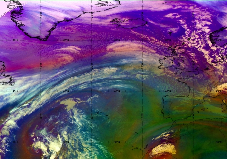
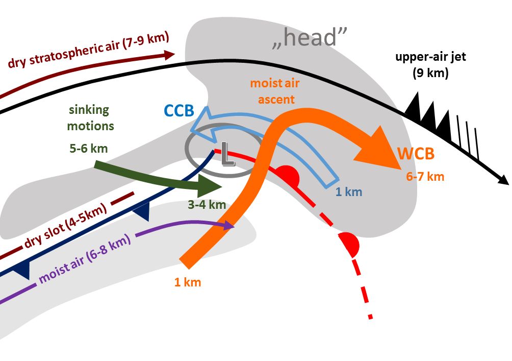
Figure 2.10:
a) Left: Airmass RGB taken on 17 January 2018 at 12 UTC.
b) Right: Idealized schematic of the flows and belts in the studied cyclone, during its developing phase on 17 January 2018, at approximately 12 UTC. The heights indicate the approximate height of the start, end or position of the depicted belts, estimated from ECMWF model output. The cloudiness is depicted schematically with grey shades. The abbreviation CCB is for Cold Conveyor Belt, and WCB for Warm Conveyor Belt. The schematic resembles the classic two-moist-conveyor-belt-and-dry-intrusion conceptual model with certain differences in the positions and heights of the belts. This structure already shows some similarities with the Shapiro-Keyser-type (e.g. onset of sinking motion at the rear of the cyclone).