Introduction
On 18 January 2018 a cyclone rapidly deepened over the British Isles and moved eastward over the Netherlands, Germany and Poland. The cyclone was accompanied by strong wind gusts, which reached 140 km/h over plains and 200 km/h over mountains (see Table 1.1 and Fig. 1.1). The windstorm caused huge damage (estimated on the order of several hundreds of millions of EUR) and also casualties.
| Station name | ASL height (m) | Country | Wind gust (km/h) |
|---|---|---|---|
| Brocken | 1142 | Germany | 205 |
| Capel Curig | 216 | UK | 150 |
| Hoek van Holland | 7 | The Netherlands | 144 |
| Gera-Lumnitz | 311 | Germany | 137 |
| Bückeburg | 70 | Germany | 126 |
| Antwerpen | 12 | Belgium | 119 |
Table 1.1: The strongest wind gusts measured on 18 January 2018 at some stations in Germany, UK, Netherland and Belgium, which were in the path of cyclone Friederike.
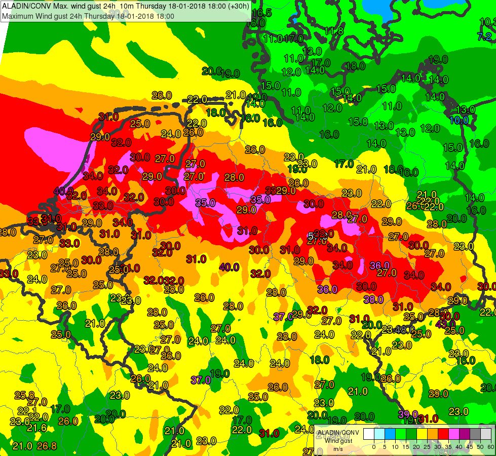
Figure 1.1: 24-hour maximum wind gust (colour, m/s) forecast from the ALADIN-HU model run initialized on 17 January 2018 at 12 UTC and valid for the period ending 18 January 2018 18 UTC. Numbers depict 24-h maximum wind gusts measured at synoptic stations and valid for the same time interval (17 January 2018 18 UTC - 18 January 2018 18 UTC) and using the same colour scale as for the model output.
Fig. 1.2 shows the cyclone at four timesteps between 16 January 18 UTC and 18 January 18 UTC, indicated by the yellow arrows.
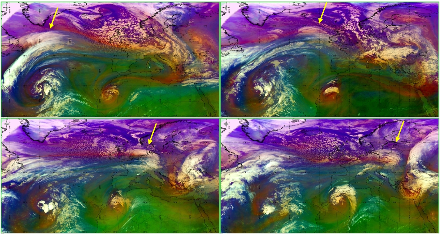
Figure 1.2: SEVIRI Airmass RGB images taken on 16 January at 18 UTC (upper left), 17 January at 12 UTC (upper right), 18 January at 06 UTC (bottom left) and 18 January at 18 UTC (bottom right). The yellow arrows indicate the cyclone under consideration.
The evolution of the cyclone can be followed on the following animation created from 6-hourly Airmass RGB images.
Animation 1: Airmass RGB Animation, 16 January 00 UTC to 19 January 06 UTC
The development of the storm could be traced with a combination of satellite (METEOSAT) imagery and NWP data (e.g. ECMWF, ALADIN). These indicated a deepening of a secondary cyclone (on the southwestern flank of a bigger, pre-existing low) and a B-type cyclogenesis (initiated by the approach of an upper-air wave to a shallow surface low in a strong upper-air-jet environment). The case also showed several interesting mesoscale features (e.g., cloud streets, wavy structures), which could be observed in the cyclone's mature phase, with the aid of high-resolution satellite imagery.
The case posed some challenges concerning both medium- and short-range forecasting. Although it was forecast several days ahead by numerical models, the deterministic runs were not consistent in predicting the intensity and character of the event. Additionally, shortly after the passage of the cyclone, the presence of a sting jet was hypothesized, based on some cloud features near the centre of the cyclone. While direct and unambiguous observational evidence of a sting jet is not available, it is possible to study the conditions for several types of instabilities and airflows using numerical models. As shown on Fig. 1.1, the strongest wind gusts (exceeding 30 m/s) occurred in an approximately 150-km-wide swath. On short timescales (+30 h), numerical models (e.g. ALADIN and ECMWF) were able to forecast the position of this swath and the intensity of the windstorm with high precision. It is, however, important to understand what physical mechanisms caused the windstorm and whether this event fits the current conceptual models of rapid cyclogenesis and related severe events.